Bootstrapping and plotting 95% confidence bands: 'Causal Inference: What If' Causal Survival Analysis
In this post, I have a look inside the Chapter 17 on Causal Survival Analysis of the “Causal Inference: What If” book by M. Hernan and J. Robins. I explore IPTW fitting following the chapter’s narrative and use the machinery of the tidyverse throughout. I utilize the script I’ve initially written in 2018. The code is not spectacularly efficient or pretty, but I deliberately did not change it 😄 There are plenty of useful open source materials for “Causal Inference: What If” book, which can be found on the
Miguel Hernan’s page.
If you are still on board, buckle up! 💨
library(tidyverse)
library(magrittr)
library(multcomp)
library(gtools)
library(survival)
library(survminer)
library(readxl)
library(wesanderson)
library(patchwork)
Getting data
temp <- tempfile()

temp2 <- tempfile()

download.file("https://cdn1.sph.harvard.edu/wp-content/uploads/sites/1268/2017/01/nhefs_excel.zip", temp)

unzip(zipfile = temp, exdir = temp2)

data <- read_xls(file.path(temp2, "NHEFS.xls"))

unlink(c(temp, temp2))
data
## # A tibble: 1,629 x 64
##     seqn  qsmk death yrdth modth dadth   sbp   dbp   sex   age  race income
##    <dbl> <dbl> <dbl> <dbl> <dbl> <dbl> <dbl> <dbl> <dbl> <dbl> <dbl>  <dbl>
##  1   233     0     0    NA    NA    NA   175    96     0    42     1     19
##  2   235     0     0    NA    NA    NA   123    80     0    36     0     18
##  3   244     0     0    NA    NA    NA   115    75     1    56     1     15
##  4   245     0     1    85     2    14   148    78     0    68     1     15
##  5   252     0     0    NA    NA    NA   118    77     0    40     0     18
##  6   257     0     0    NA    NA    NA   141    83     1    43     1     11
##  7   262     0     0    NA    NA    NA   132    69     1    56     0     19
##  8   266     0     0    NA    NA    NA   100    53     1    29     0     22
##  9   419     0     1    84    10    13   163    79     0    51     0     18
## 10   420     0     1    86    10    17   184   106     0    43     0     16
## # … with 1,619 more rows, and 52 more variables: marital <dbl>, school <dbl>,
## #   education <dbl>, ht <dbl>, wt71 <dbl>, wt82 <dbl>, wt82_71 <dbl>,
## #   birthplace <dbl>, smokeintensity <dbl>, smkintensity82_71 <dbl>,
## #   smokeyrs <dbl>, asthma <dbl>, bronch <dbl>, tb <dbl>, hf <dbl>, hbp <dbl>,
## #   pepticulcer <dbl>, colitis <dbl>, hepatitis <dbl>, chroniccough <dbl>,
## #   hayfever <dbl>, diabetes <dbl>, polio <dbl>, tumor <dbl>,
## #   nervousbreak <dbl>, alcoholpy <dbl>, alcoholfreq <dbl>, alcoholtype <dbl>,
## #   alcoholhowmuch <dbl>, pica <dbl>, headache <dbl>, otherpain <dbl>,
## #   weakheart <dbl>, allergies <dbl>, nerves <dbl>, lackpep <dbl>,
## #   hbpmed <dbl>, boweltrouble <dbl>, wtloss <dbl>, infection <dbl>,
## #   active <dbl>, exercise <dbl>, birthcontrol <dbl>, pregnancies <dbl>,
## #   cholesterol <dbl>, hightax82 <dbl>, price71 <dbl>, price82 <dbl>,
## #   tax71 <dbl>, tax82 <dbl>, price71_82 <dbl>, tax71_82 <dbl>
Section 17.1
For this section I partly re-used the code by Joy Shi and Sean McGrath available here.
# define/recode variables
data %<>%
  mutate(
    # define censoring
    cens = if_else(is.na(wt82_71),1, 0),
    # categorize the school variable (as in R code by Joy Shi and Sean McGrath)
    education = cut(school, breaks = c(0, 8, 11, 12, 15, 20),
                    include.lowest = TRUE,
                    labels = c('1. 8th Grage or Less',
                               '2. HS Dropout',
                               '3. HS',
                               '4. College Dropout',
                               '5. College or More')),
    # establish active as a factor variable
    active = factor(active),
    # establish exercise as a factor variable
    exercise = factor(exercise),
    # create a treatment label variable
    qsmklabel = if_else(qsmk == 1,
                        'Quit Smoking 1971-1982',
                        'Did Not Quit Smoking 1971-1982'),
  # survtime variable
  survtime = if_else(death == 0, 120, (yrdth-83)*12 + modth) # yrdth ranges from 83 to 92
    ) %>%
  # ignore those with missing values on some variables
  filter(!is.na(education))
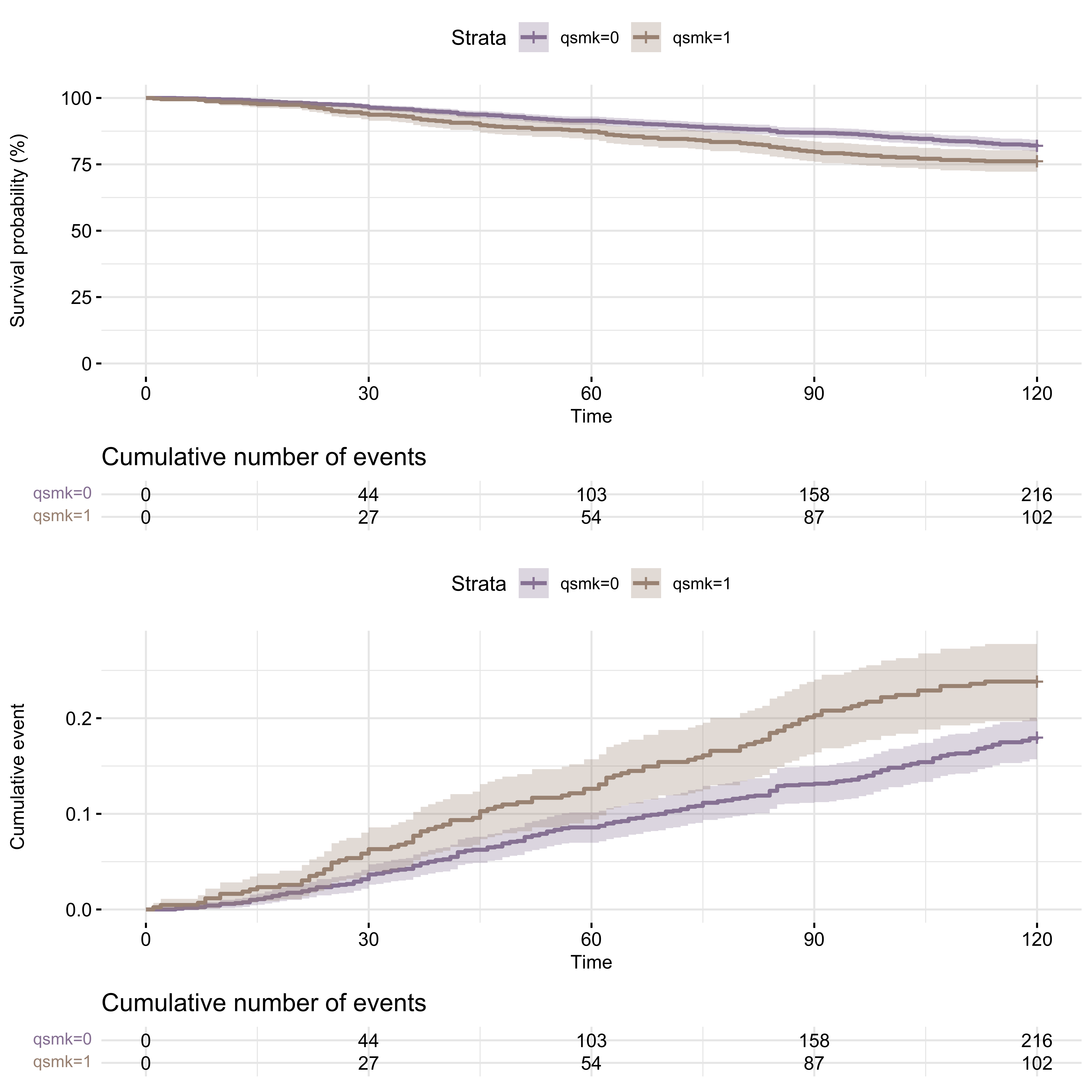
First, I go along with the survminer package functionality and plot Kaplan-Meier survival curves for smokers vs non-smokers and Kaplan-Meier cumulative mortality curves for smokers vs non-smokers.
# fit a Kaplan-Meier (KM) survival model: non-parametric
# survfit function creates survival curves from either a formula (e.g. the Kaplan-Meier), a previously fitted Cox model, or a previously fitted accelerated failure time model
fit_surv <- survfit(Surv(time = survtime, event = death) ~ qsmk, data = data)

fit_surv_tidy <- fit_surv %>% broom::tidy(., conf.int = T)

fit_surv_tidy
## # A tibble: 169 x 9
##     time n.risk n.event n.censor estimate std.error conf.high conf.low strata
##    <dbl>  <dbl>   <dbl>    <dbl>    <dbl>     <dbl>     <dbl>    <dbl> <chr>
##  1     4   1201       1        0    0.999  0.000833     1        0.998 qsmk=0
##  2     5   1200       1        0    0.998  0.00118      1        0.996 qsmk=0
##  3     7   1199       1        0    0.998  0.00144      1        0.995 qsmk=0
##  4     8   1198       2        0    0.996  0.00187      0.999    0.992 qsmk=0
##  5    10   1196       2        0    0.994  0.00221      0.998    0.990 qsmk=0
##  6    12   1194       1        0    0.993  0.00236      0.998    0.989 qsmk=0
##  7    13   1193       1        0    0.993  0.00251      0.997    0.988 qsmk=0
##  8    14   1192       3        0    0.990  0.00290      0.996    0.984 qsmk=0
##  9    15   1189       1        0    0.989  0.00302      0.995    0.983 qsmk=0
## 10    16   1188       2        0    0.988  0.00325      0.994    0.981 qsmk=0
## # … with 159 more rows
# Figure 17.1, p. 70, Part II
figure_17.1 <- ggsurvplot(fit_surv,
           fun = "pct",
           conf.int = TRUE,
           ggtheme = theme_minimal(),
           palette = c("#9986A5", "#AA9486"), # wesanderson package IsleofDogs2 theme
           cumevents = T,
           cumcensor = F,
           tables.height = 0.2,
           tables.theme = theme_cleantable(),
           font.main = c(10, "bold", "black"),
           font.x = c(10, "plain", "black"),
           font.y = c(10, "plain", "black"),
           font.tickslab = c(10, "plain", "black"),
           fontsize = 3.5,
           data = data)

# KM model 1-survival
figure_17.1_cumevent <- ggsurvplot(fit = fit_surv,
           fun = "event",
           conf.int = TRUE,
           ggtheme = theme_minimal(),
           palette = c("#9986A5", "#AA9486"), # wesanderson package IsleofDogs2 theme
           cumevents = T,
           cumcensor = F,
           tables.height = 0.2,
           tables.theme = theme_cleantable(),
           font.main = c(10, "plain", "black"),
           font.x = c(10, "plain", "black"),
           font.y = c(10, "plain", "black"),
           font.tickslab = c(10, "plain", "black"),
           fontsize = 3.5,
           data = data)

# combine survminer plots
arrange_ggsurvplots(list(figure_17.1, figure_17.1_cumevent), print = TRUE, ncol = 1, nrow = 2)
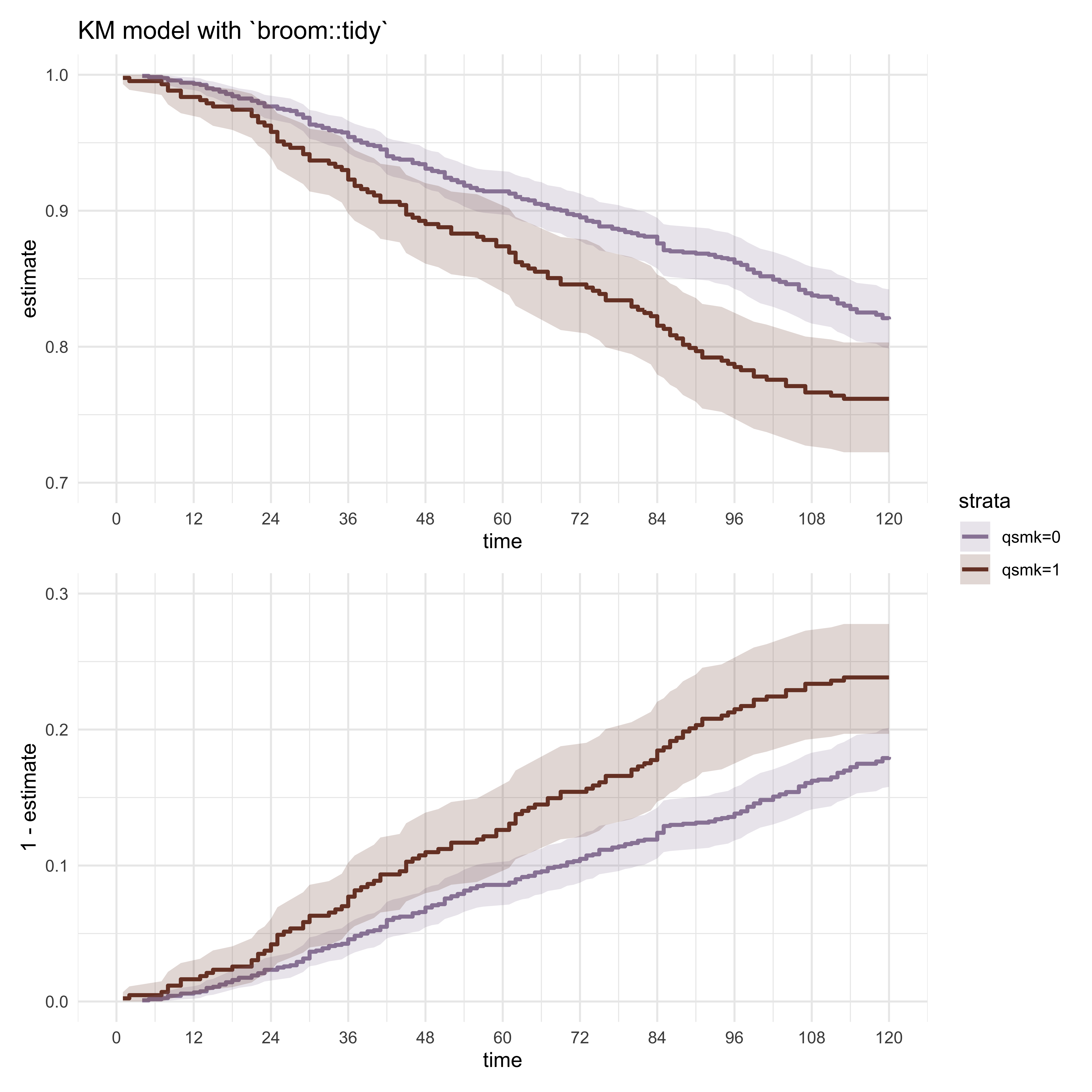
Although I find survminer package to be a great tool and sufficiently flexible one too, sometimes I need full-ish control over my survival or 1-survival plots. For these occasions, I use broom and ggplot2 functionality together. I also discovered patchwork package some time ago and since that moment I use it every time I want to combine several plots in one. Here is the re-make of the survminer visualization of KM plots.
# KM: alternative plots with tidy + patchwork

risk.table <- fit_surv_tidy %>%
  group_by(strata) %>%
  rownames_to_column() %>%
  gather(var, value, -rowname) %>% # since it is an old-ish code I used gather and spread, now one could use `pivot_wider`
  spread(rowname, value)

p1_km <- fit_surv_tidy %>%
  group_by(strata) %>%
  ggplot(aes(x = time, y = estimate, color = strata, fill = strata)) +
  geom_step(size = 1) +
  scale_x_continuous(limits = c(0, 120), breaks = seq(0, 120, 12)) +
  scale_y_continuous(limits = c(0.7, 1)) +
  geom_ribbon(aes(ymin = conf.low, ymax = conf.high), alpha = .2, colour = NA) +
  theme_minimal() +
  ggtitle("KM model with `broom::tidy`") +
  scale_fill_manual(values = wes_palette("IsleofDogs1")) +
  scale_color_manual(values = wes_palette("IsleofDogs1"))

# KM: 1-survival
p2_km <- fit_surv_tidy %>% group_by(strata) %>% ggplot(aes(x = time, y = 1 - estimate, color = strata, fill = strata)) +
  geom_step(size = 1) +
  scale_x_continuous(limits = c(0, 120), breaks = seq(0, 120, 12)) +
  scale_y_continuous(limits = c(0, 0.3)) +
  geom_ribbon(aes(ymax = 1 - conf.low, ymin = 1 - conf.high), alpha = .2, colour = NA) +
  theme_minimal() +
  scale_fill_manual(values = wes_palette("IsleofDogs1")) +
  scale_color_manual(values = wes_palette("IsleofDogs1"))
# combined figures
p1_km + p2_km +
  plot_layout(nrow = 2, guides = "collect")
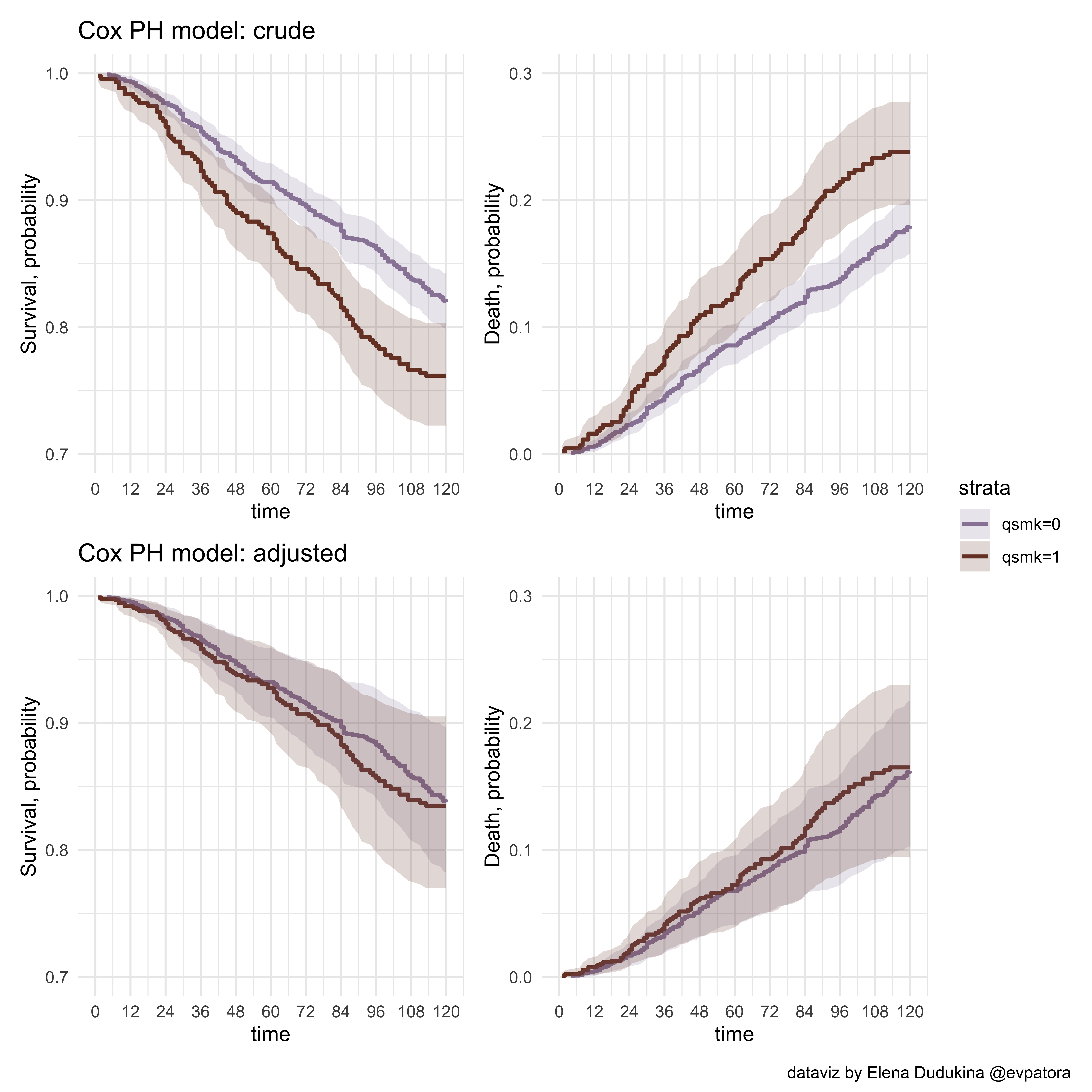
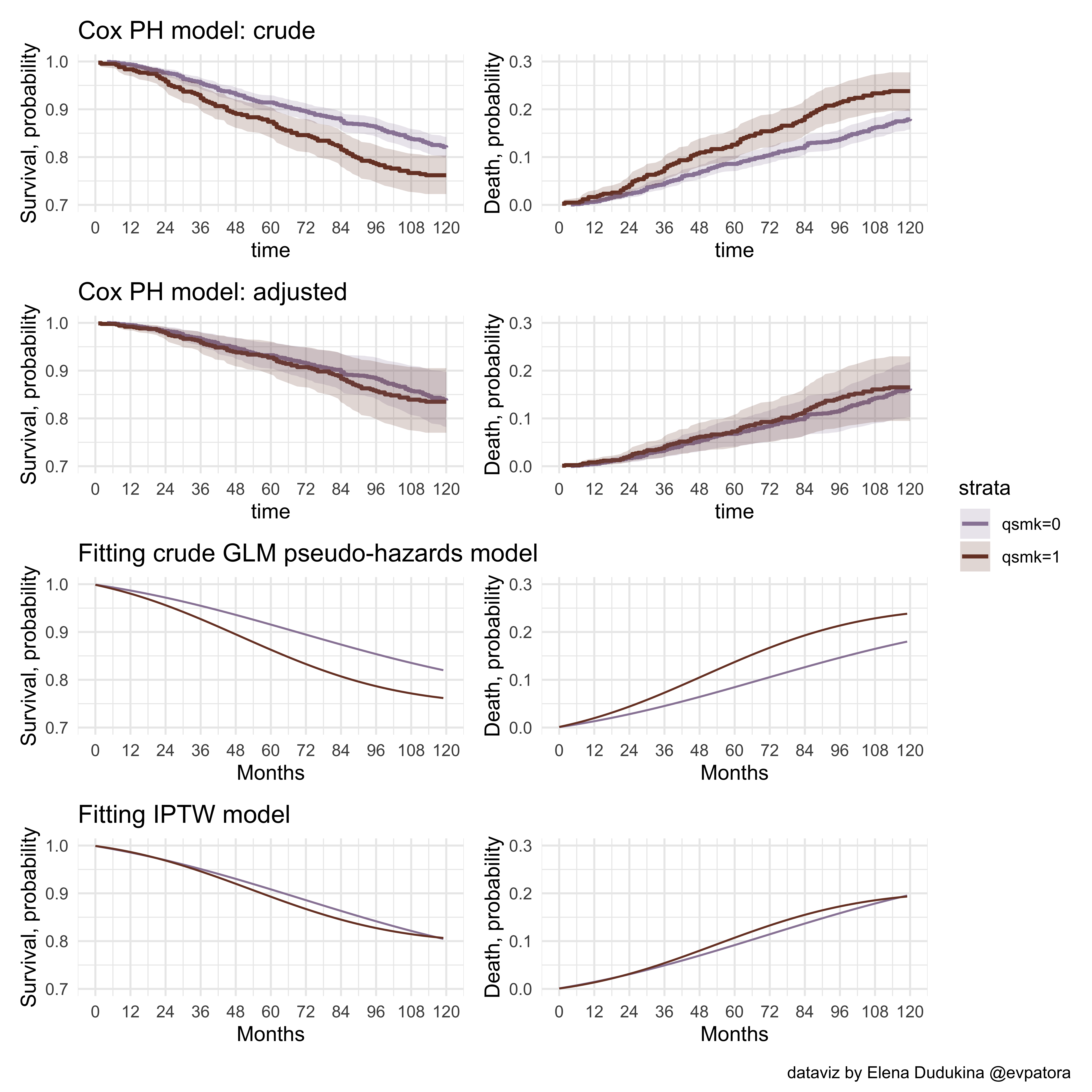
Next, I create the survival and cumulative events plots using crude and adjusted Cox proportional hazards models for the sake of doing it 😅
# Cox PH: crude (same results as with KM model)
cox_model <- survfit(coxph(Surv(survtime, death) ~ strata(qsmk), data = data))

cox_fit_crude <- cox_model %>% broom::tidy(., conf.int = T, exponentiate = T)

# survival
cox_crude_p1 <- cox_fit_crude %>%
  group_by(strata) %>%
  ggplot(aes(x = time, y = estimate, color = strata, fill = strata)) +
  geom_step(size = 1) +
  scale_x_continuous(limits = c(0, 120), breaks = seq(0, 120, 12)) +
  scale_y_continuous(limits = c(0.7, 1)) +
  ylab("Survival, probability") +
  geom_ribbon(aes(ymin = conf.low, ymax = conf.high), alpha = .2, colour = NA) +
  theme_minimal() +
  ggtitle("Cox PH model: crude") +
  scale_fill_manual(values = wes_palette("IsleofDogs1")) +
  scale_color_manual(values = wes_palette("IsleofDogs1"))

# 1-survival
cox_crude_p2 <- cox_fit_crude %>%
  group_by(strata) %>%
  ggplot(aes(x = time, y = 1 - estimate, color = strata, fill = strata)) +
  geom_step(size = 1) +
  scale_x_continuous(limits = c(0, 120), breaks = seq(0, 120, 12)) +
  scale_y_continuous(limits = c(0, 0.3)) +
  ylab("Death, probability") +
  geom_ribbon(aes(ymax = 1 - conf.low, ymin = 1 - conf.high), alpha = .2, colour = NA) +
  theme_minimal() +
  scale_fill_manual(values = wes_palette("IsleofDogs1")) +
  scale_color_manual(values = wes_palette("IsleofDogs1"))

# Cox PH : adjusted
cox_model2 <- survfit(coxph(Surv(survtime, death) ~ strata(qsmk) + sex + race + age + I(age*age)
                + as.factor(education) + smokeintensity
                + I(smokeintensity*smokeintensity) + smkintensity82_71
                + smokeyrs + I(smokeyrs*smokeyrs) + as.factor(exercise)
                + as.factor(active) + wt71 + I(wt71*wt71), data = data))

cox_fit_adj <- cox_model2 %>% broom::tidy(., conf.int = T, exponentiate = T)

# survival
cox_adj_p1 <- cox_fit_adj %>%
  group_by(strata) %>%
  ggplot(aes(x = time, y = estimate, color = strata, fill = strata)) +
  geom_step(size = 1) +
  scale_x_continuous(limits = c(0, 120), breaks = seq(0, 120, 12)) +
  scale_y_continuous(limits = c(0.7, 1)) +
  ylab("Survival, probability") +
  geom_ribbon(aes(ymin = conf.low, ymax = conf.high), alpha = .2, colour = NA) +
  theme_minimal() +
  ggtitle("Cox PH model: adjusted") +
  scale_fill_manual(values = wes_palette("IsleofDogs1")) +
  scale_color_manual(values = wes_palette("IsleofDogs1"))

# 1-survival
cox_adj_p2 <- cox_fit_adj %>%
  group_by(strata) %>%
  ggplot(aes(x = time, y = 1 - estimate, color = strata, fill = strata)) +
  geom_step(size = 1) +
  scale_x_continuous(limits = c(0, 120), breaks = seq(0, 120, 12)) +
  scale_y_continuous(limits = c(0, 0.3)) +
  ylab("Death, probability") +
  geom_ribbon(aes(ymax = 1 - conf.low, ymin = 1 - conf.high), alpha = .2, colour = NA) +
  theme_minimal() +
  scale_fill_manual(values = wes_palette("IsleofDogs1")) +
  scale_color_manual(values = wes_palette("IsleofDogs1"))
# combined figure
cox_crude_p1 + cox_crude_p2 + cox_adj_p1 + cox_adj_p2 +
  plot_layout(ncol = 2, guides = "collect") +
  plot_annotation(
  caption = "dataviz by Elena Dudukina @evpatora"
)
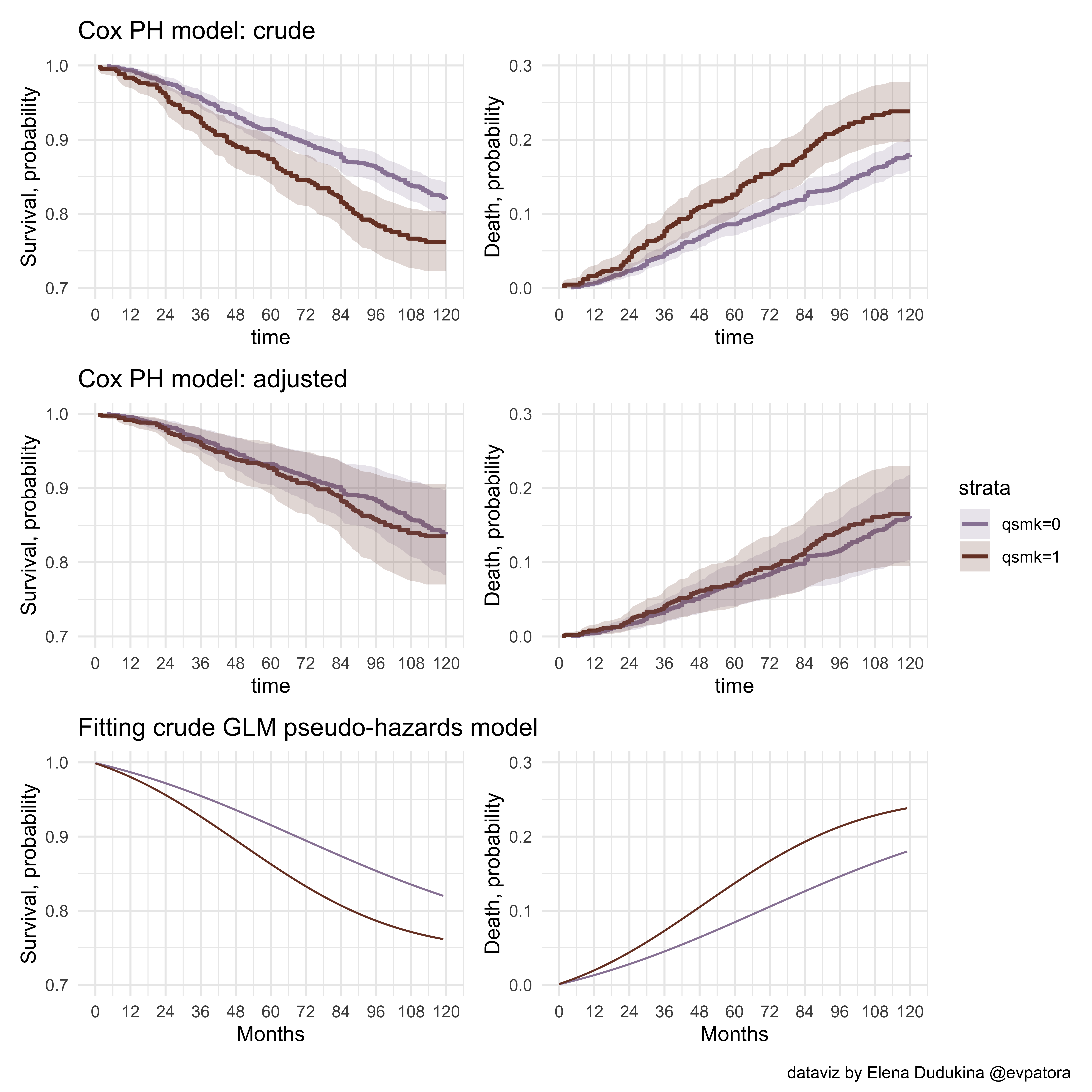
Section 17.2
For this section, I create the observation-month data following the “What If” Chapter 17 narrative.
# CRUDE GLM hazard model
# create month data
months <- data[rep(1:nrow(data), times = data$survtime), ]

# each participant now has the rows for all months of the follow-up
months
## # A tibble: 176,764 x 67
##     seqn  qsmk death yrdth modth dadth   sbp   dbp   sex   age  race income
##    <dbl> <dbl> <dbl> <dbl> <dbl> <dbl> <dbl> <dbl> <dbl> <dbl> <dbl>  <dbl>
##  1   233     0     0    NA    NA    NA   175    96     0    42     1     19
##  2   233     0     0    NA    NA    NA   175    96     0    42     1     19
##  3   233     0     0    NA    NA    NA   175    96     0    42     1     19
##  4   233     0     0    NA    NA    NA   175    96     0    42     1     19
##  5   233     0     0    NA    NA    NA   175    96     0    42     1     19
##  6   233     0     0    NA    NA    NA   175    96     0    42     1     19
##  7   233     0     0    NA    NA    NA   175    96     0    42     1     19
##  8   233     0     0    NA    NA    NA   175    96     0    42     1     19
##  9   233     0     0    NA    NA    NA   175    96     0    42     1     19
## 10   233     0     0    NA    NA    NA   175    96     0    42     1     19
## # … with 176,754 more rows, and 55 more variables: marital <dbl>, school <dbl>,
## #   education <fct>, ht <dbl>, wt71 <dbl>, wt82 <dbl>, wt82_71 <dbl>,
## #   birthplace <dbl>, smokeintensity <dbl>, smkintensity82_71 <dbl>,
## #   smokeyrs <dbl>, asthma <dbl>, bronch <dbl>, tb <dbl>, hf <dbl>, hbp <dbl>,
## #   pepticulcer <dbl>, colitis <dbl>, hepatitis <dbl>, chroniccough <dbl>,
## #   hayfever <dbl>, diabetes <dbl>, polio <dbl>, tumor <dbl>,
## #   nervousbreak <dbl>, alcoholpy <dbl>, alcoholfreq <dbl>, alcoholtype <dbl>,
## #   alcoholhowmuch <dbl>, pica <dbl>, headache <dbl>, otherpain <dbl>,
## #   weakheart <dbl>, allergies <dbl>, nerves <dbl>, lackpep <dbl>,
## #   hbpmed <dbl>, boweltrouble <dbl>, wtloss <dbl>, infection <dbl>,
## #   active <fct>, exercise <fct>, birthcontrol <dbl>, pregnancies <dbl>,
## #   cholesterol <dbl>, hightax82 <dbl>, price71 <dbl>, price82 <dbl>,
## #   tax71 <dbl>, tax82 <dbl>, price71_82 <dbl>, tax71_82 <dbl>, cens <dbl>,
## #   qsmklabel <chr>, survtime <dbl>
# for each person in the dataset
months %<>%
  group_by(seqn) %>%
  # set time to start from 0 month
  mutate (
  time = row_number() - 1,
  # create event variable
  event = case_when(
    time == survtime - 1 & death == 1 ~ 1,
    TRUE ~ 0
  ),
  # time squared term
  timesq = time*time
  ) %>%
  ungroup()

# fit crude GLM hazards model: the model for not-event
hazard_mod1 <- glm(family = binomial(link = "logit"), data = months, event == 0 ~ qsmk + qsmk*time + qsmk*timesq + time + timesq)

# tidy results
hazard_mod1_tidy <- hazard_mod1 %>% broom::tidy(., conf.int = T, exponentiate = T)

hazard_mod1_tidy[, c(1, 2, 3, 6, 7)]
## # A tibble: 6 x 5
##   term        estimate std.error conf.low conf.high
##   <chr>          <dbl>     <dbl>    <dbl>     <dbl>
## 1 (Intercept) 1092.    0.231      708.     1754.
## 2 qsmk           0.715 0.397        0.334     1.59
## 3 time           0.981 0.00841      0.964     0.997
## 4 timesq         1.00  0.0000669    1.00      1.00
## 5 qsmk:time      0.988 0.0150       0.959     1.02
## 6 qsmk:timesq    1.00  0.000125     1.00      1.00
# create the dataset with all time points/all observation-months under each treatment level (treated, untreated)
months0 <- tibble(time = seq(0, 119),
                qsmk = 0, # untreated
                timesq = seq(0, 119)^2)

months1 <- tibble(time = seq(0, 119),
                qsmk = 1, # treated
                timesq = seq(0, 119)^2)

# predict 1-hazard to each observation-month; NB: newdata argument
months0 %<>%
  mutate(
    p.not.event = predict(hazard_mod1, type = "response", newdata = months0)
  )

# quick summary
summary(months0$p.not.event)
##    Min. 1st Qu.  Median    Mean 3rd Qu.    Max.
##  0.9980  0.9981  0.9982  0.9983  0.9985  0.9991
months1 %<>%
  mutate(
    p.not.event = predict(hazard_mod1, type = "response", newdata = months1)
  )

# quick summary
summary(months1$p.not.event)
##    Min. 1st Qu.  Median    Mean 3rd Qu.    Max.
##  0.9969  0.9971  0.9976  0.9977  0.9983  0.9990
# compute survival for each observation-month
months0 %<>%
  mutate(
    # to find a cumulative probability of not-event take a cumulative product of probabilities
    p.surv = cumprod(p.not.event)
  )

# quick summary
summary(months0$p.surv)
##    Min. 1st Qu.  Median    Mean 3rd Qu.    Max.
##  0.8201  0.8648  0.9164  0.9139  0.9640  0.9991
months1 %<>%
  mutate(
    # to find a cumulative probability of not-event take a cumulative product of probabilities
    p.surv = cumprod(p.not.event)
  )

# quick summary
summary(months1$p.surv)
##    Min. 1st Qu.  Median    Mean 3rd Qu.    Max.
##  0.7618  0.7974  0.8642  0.8709  0.9427  0.9987
# difference in survival in each observation month
surv_diff <- bind_cols(months0, months1[, "p.surv"]) %>%
  mutate(
    surv_diff = p.surv...6 - p.surv...5
  )
## New names:
## * p.surv -> p.surv...5
## * p.surv -> p.surv...6
# bind and plot
months_plot <- bind_rows(months0, months1)

p1_glm_1 <- months_plot %>%
  group_by(qsmk) %>%
  ggplot(aes(x = time, y = p.surv, color = factor(qsmk), fill = factor(qsmk))) +
  geom_line() +
  xlab("Months") +
  scale_x_continuous(limits = c(0, 120), breaks = seq(0, 120, 12)) +
  scale_y_continuous(limits = c(0.7, 1), breaks = seq(0.7, 1, 0.1)) +
  ylab("Survival, probability") +
  ggtitle("Fitting crude GLM pseudo-hazards model") +
  theme_minimal() +
  theme(legend.position = "none") +
  labs(colour = "Smoking", fill = "Smoking") +
  scale_fill_manual(values = wes_palette("IsleofDogs1")) +
  scale_color_manual(values = wes_palette("IsleofDogs1"))

# 1-survival
p1_glm_2 <- months_plot %>%
  group_by(qsmk) %>%
  ggplot(aes(x = time, y = 1 - p.surv, color = factor(qsmk), fill = factor(qsmk))) +
  geom_line() +
  xlab("Months") +
  scale_x_continuous(limits = c(0, 120), breaks = seq(0, 120, 12)) +
  scale_y_continuous(limits = c(0, 0.3), breaks = seq(0, 0.3, 0.1)) +
  ylab("Death, probability") +
  ggtitle("") +
  theme_minimal() +
  theme(legend.position = "none") +
  labs(colour = "Smoking", fill = "Smoking") +
  scale_fill_manual(values = wes_palette("IsleofDogs1")) +
  scale_color_manual(values = wes_palette("IsleofDogs1"))

p1_glm_3 <- surv_diff %>%
  ggplot(aes(x = time, y = surv_diff)) +
  geom_line() +
  xlab("Months") +
  ylab("Difference") +
  ggtitle("") +
  theme_minimal()+
  labs(colour = "Smoking", fill = "Smoking") +
  scale_x_continuous(limits = c(0, 120), breaks = seq(0, 120, 12)) +
  scale_fill_manual(values = wes_palette("IsleofDogs1")) +
  scale_color_manual(values = wes_palette("IsleofDogs1"))
# combine plots
comb <- cox_crude_p1 + cox_crude_p2 + cox_adj_p1 + cox_adj_p2 + p1_glm_1 + p1_glm_2 +
  plot_layout(ncol = 2, guides = "collect")  +
  plot_annotation(
  caption = "dataviz by Elena Dudukina @evpatora"
)
comb
Section 17.3
In this section, I apply GLM model for the average treatment effect (ATE) of smoking on the mortality using inverse probability of treatment weighting (IPTW) and tackle confounding by age, sex, ethnicity, education, smoking intensity and duration, exercising, daily activity, and weights in 1971.
# model numerator and denominator for computing stabilized IPTW
# numerator
ipw_num <- glm(qsmk ~ 1, data = data, family = binomial(link = "logit"))
# denominator (propensity score model for the treatment)
ipw_denom <- glm(qsmk ~ sex + race + age + I(age*age) + as.factor(education) + smokeintensity + I(smokeintensity*smokeintensity) + smokeyrs + I(smokeyrs*smokeyrs) + as.factor(exercise) + as.factor(active) + wt71 + I(wt71*wt71), data = data, family = binomial(link = "logit"))
# update the dataset with the predicted probabilities of the treatment in the treated and in the untreated
data %<>% mutate(
# predicted probability of the treatment for ATE: marginal probability of the treatment
p_x = predict(ipw_num, type = "response"),
# for exposed and unexposed
p_x = case_when(
qsmk == 1 ~ p_x,
is.na(qsmk) ~ NA_real_,
TRUE ~ 1 - p_x
),
# predicted probability of the treatment for ATE: probability of treatment given confounders
p_x_l = predict(ipw_denom, type = "response"),
# for exposed and unexposed
p_x_l = case_when(
qsmk == 1 ~ p_x_l,
is.na(qsmk) ~ NA_real_,
TRUE ~ 1-p_x_l
),
# stabilized IPTW
iptw_stab = p_x / p_x_l
)
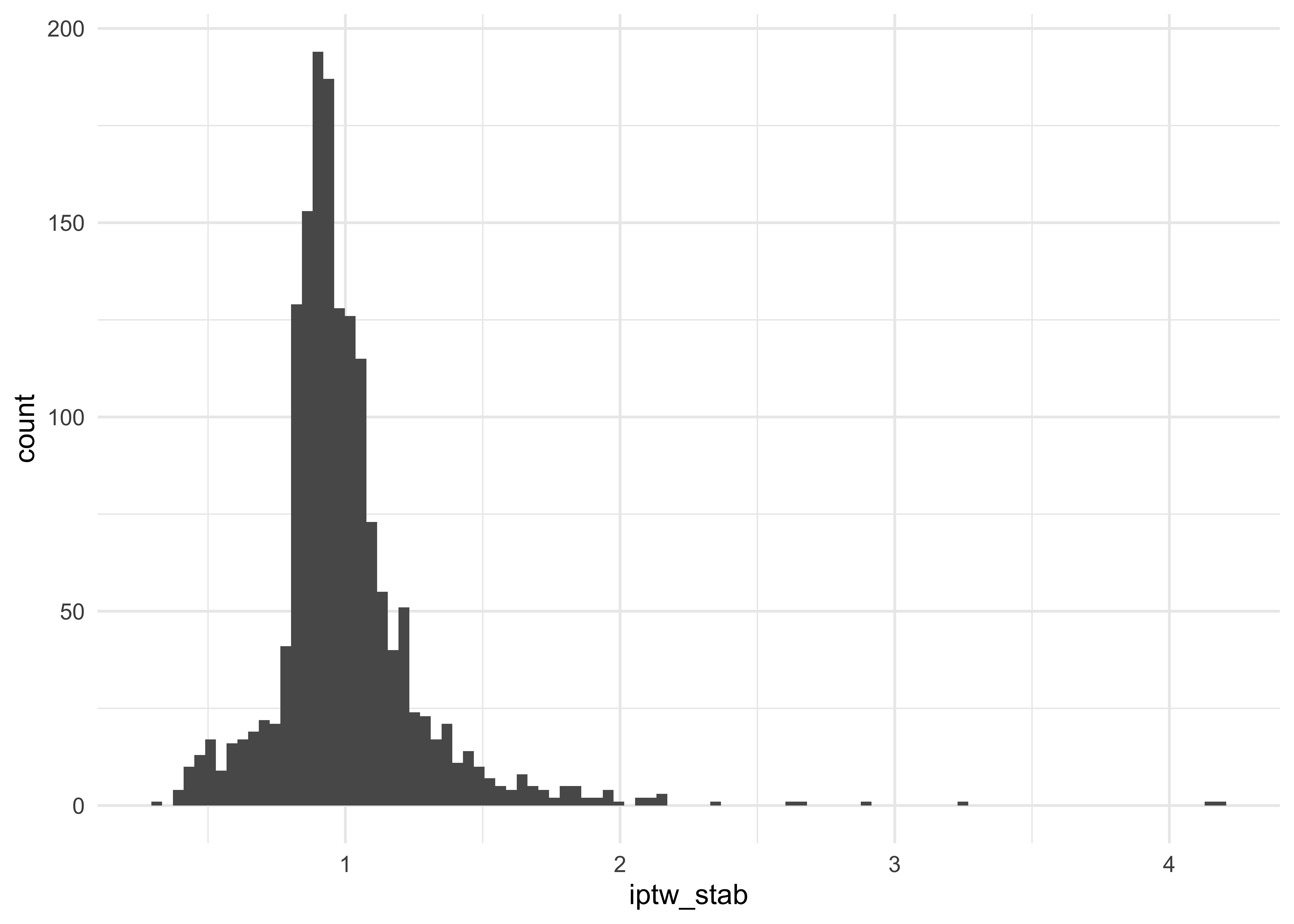
# check stabilized IPTW distribution
data %>%
dplyr::select(iptw_stab) %>%
summarise_all(.funs = list(
Q25 = ~quantile(., probs = 0.25),
median = ~quantile(., probs = 0.5),
Q75 = ~quantile(., probs = 0.75),
min = min,
mean = mean,
max = max)) %>%
kableExtra::kable(format = "html")
| Q25 | median | Q75 | min | mean | max |
|---|---|---|---|---|---|
| 0.8639949 | 0.9503936 | 1.075472 | 0.3312358 | 0.9990652 | 4.205432 |
# check of stabilized IPTW distribution graphically
data %>%
  ggplot(aes(x = iptw_stab)) +
  geom_histogram(bins = 100) +
  theme_minimal()
# create month data for the IPTW analysis
months_iptw <- data[rep(1:nrow(data), times = data$survtime),]

months_iptw %<>%
  group_by(seqn) %>%
  mutate (
    time = row_number() - 1,
    event = case_when(
      time == survtime -1 & death == 1 ~ 1,
      TRUE ~ 0
    ),
    timesq = time*time
  ) %>%
  ungroup()


# check IPTW
months_iptw %>%
  dplyr::select(iptw_stab) %>%
  summarise_all(.funs = list(
    Q25 = ~quantile(., probs = 0.25),
    median = ~quantile(., probs = 0.5),
    Q75 = ~quantile(., probs = 0.75),
    min = min,
    mean = mean,
    max = max))
## # A tibble: 1 x 6
##     Q25 median   Q75   min  mean   max
##   <dbl>  <dbl> <dbl> <dbl> <dbl> <dbl>
## 1 0.867  0.948  1.07 0.331  1.00  4.21
# IPTW model: glm
ipw_model <- glm(event == 0 ~ qsmk + qsmk*time + qsmk*timesq + time + timesq, family = binomial(link = "logit"), weight = iptw_stab, data = months_iptw)

ipw_model %>%
  broom::tidy(., conf.int = T, exponentiate = T)
## # A tibble: 6 x 7
##   term        estimate std.error statistic   p.value conf.low conf.high
##   <chr>          <dbl>     <dbl>     <dbl>     <dbl>    <dbl>     <dbl>
## 1 (Intercept)  989.    0.221        31.2   2.87e-214  654.     1555.
## 2 qsmk           1.20  0.440         0.408 6.83e-  1    0.521     2.95
## 3 time           0.981 0.00805      -2.35  1.90e-  2    0.966     0.997
## 4 timesq         1.00  0.0000640     1.85  6.49e-  2    1.00      1.00
## 5 qsmk:time      0.981 0.0164       -1.16  2.48e-  1    0.949     1.01
## 6 qsmk:timesq    1.00  0.000135      1.56  1.20e-  1    1.00      1.00
# create the dataset with all time points/all observation-months_iptw under each treatment level (treated, untreated)
months0_iptw <- tibble(time = seq(0, 119),
                  qsmk = 0,
                  timesq = seq(0, 119)^2)

months1_iptw <- tibble(time = seq(0, 119),
                  qsmk = 1,
                  timesq = seq(0, 119)^2)

# assign estimated 1-"hazard" to each observation-month; NB: newdata argument
months0_iptw %<>%
  mutate(
    p.not.event = predict(ipw_model, type = "response", newdata = months0_iptw)
  )

summary(months0_iptw$p.not.event)
##    Min. 1st Qu.  Median    Mean 3rd Qu.    Max.
##  0.9979  0.9979  0.9981  0.9982  0.9984  0.9990
months1_iptw %<>%
  mutate(
    p.not.event = predict(ipw_model, type = "response", newdata = months1_iptw)
  )

summary(months1_iptw$p.not.event)
##    Min. 1st Qu.  Median    Mean 3rd Qu.    Max.
##  0.9975  0.9977  0.9981  0.9982  0.9987  0.9993
# compute survival for each observation-month
months0_iptw %<>%
  mutate(
    # to find a cumulative probability of not-event take a cumulative product of probabilities
    p.surv = cumprod(p.not.event)
  )
summary(months0_iptw$p.surv)
##    Min. 1st Qu.  Median    Mean 3rd Qu.    Max.
##  0.8047  0.8536  0.9093  0.9066  0.9607  0.9990
months1_iptw %<>%
  mutate(
    # to find a cumulative probability of not-event take a cumulative product of probabilities
    p.surv = cumprod(p.not.event)
  )
summary(months1_iptw$p.surv)
##    Min. 1st Qu.  Median    Mean 3rd Qu.    Max.
##  0.8067  0.8367  0.8941  0.8979  0.9583  0.9992
# difference in survival in each observation month (for later)
surv_diff_iptw <- bind_cols(months0_iptw, months1_iptw[, "p.surv"]) %>%
  mutate(
    surv_diff_iptw = p.surv...6 - p.surv...5
  )
## New names:
## * p.surv -> p.surv...5
## * p.surv -> p.surv...6
# bind and plot
surv_diff_iptw <- bind_rows(months0_iptw, months1_iptw)

p_iptw_1 <- surv_diff_iptw %>%
  group_by(qsmk) %>%
  ggplot(aes(x = time, y = p.surv, color = factor(qsmk), fill = factor(qsmk))) +
  geom_line() +
  xlab("Months") +
  scale_x_continuous(limits = c(0, 120), breaks = seq(0,120,12)) +
  scale_y_continuous(limits = c(0.7, 1), breaks = seq(0.7, 1, 0.1)) +
  ylab("Survival, probability") +
  ggtitle("Fitting IPTW model") +
  theme_minimal() +
  theme(legend.position = "none") +
  scale_fill_manual(values = wes_palette("IsleofDogs1")) +
  scale_color_manual(values = wes_palette("IsleofDogs1"))

# 1-survival: IPTW model
p_iptw_2 <- surv_diff_iptw %>%
  group_by(qsmk) %>%
  ggplot(aes(x = time, y = 1 - p.surv, color = factor(qsmk), fill = factor(qsmk))) +
  geom_line() +
  scale_x_continuous(limits = c(0, 120), breaks = seq(0, 120, 12)) +
  scale_y_continuous(limits = c(0, 0.3), breaks = seq(0, 0.3, 0.1)) +
  xlab("Months") +
  ylab("Death, probability") +
  theme_minimal() +
  theme(legend.position = "none") +
  scale_fill_manual(values = wes_palette("IsleofDogs1")) +
  scale_color_manual(values = wes_palette("IsleofDogs1"))
# combine plots
cox_crude_p1 + cox_crude_p2 + cox_adj_p1 + cox_adj_p2 + p1_glm_1 + p1_glm_2 + p_iptw_1 + p_iptw_2 +
  plot_layout(ncol = 2, guides = "collect") +
  plot_annotation(
  caption = "dataviz by Elena Dudukina @evpatora"
)
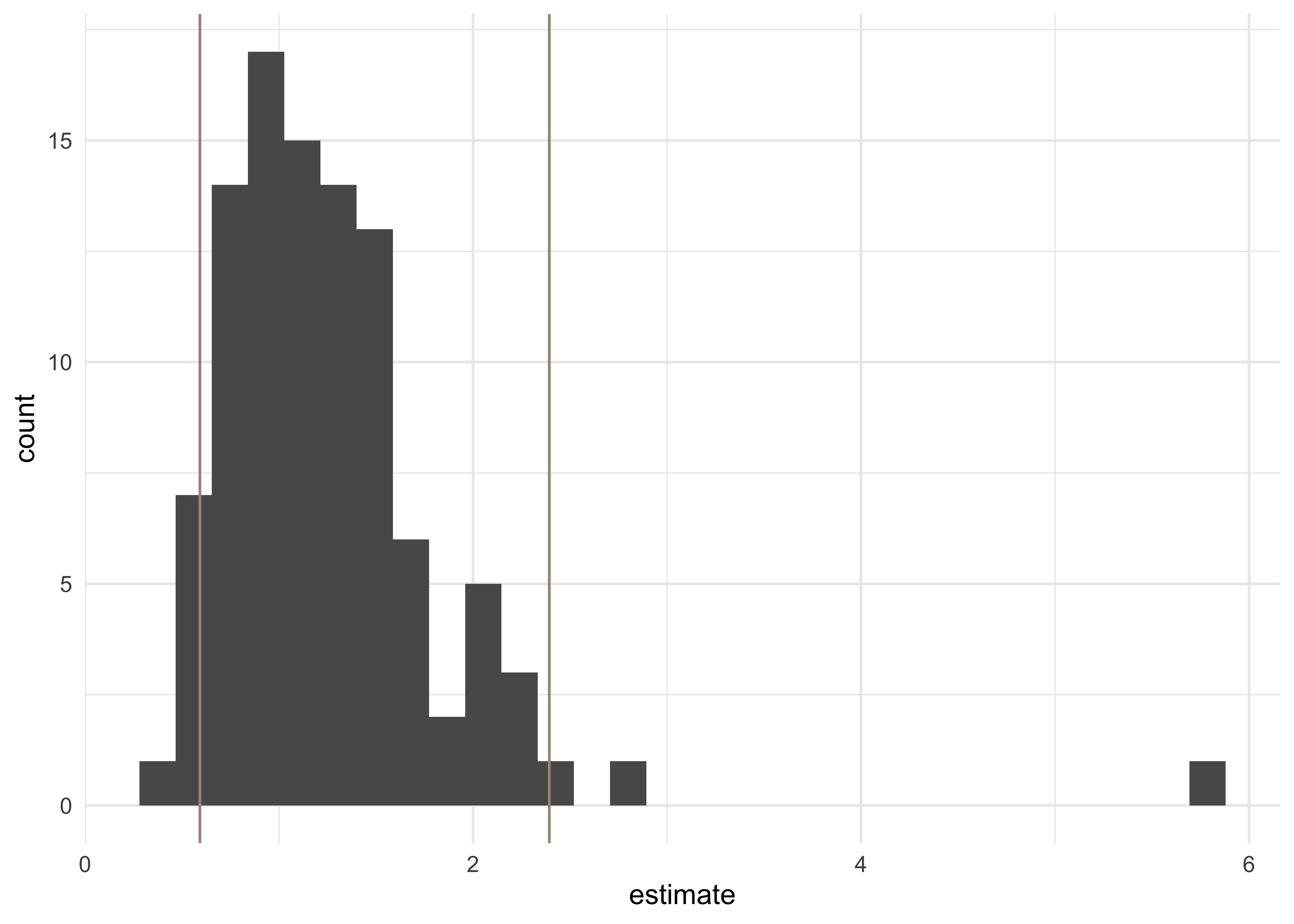
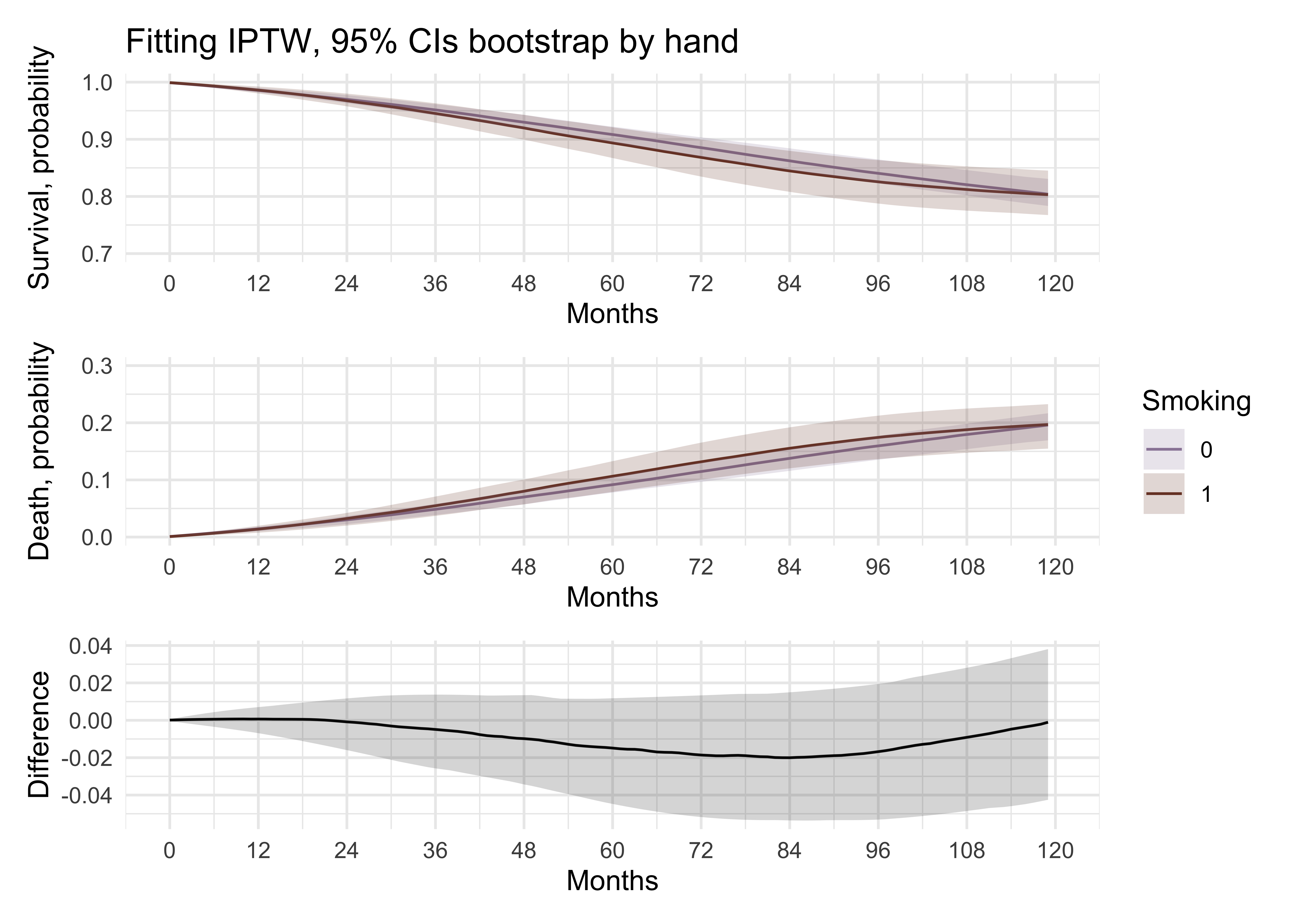
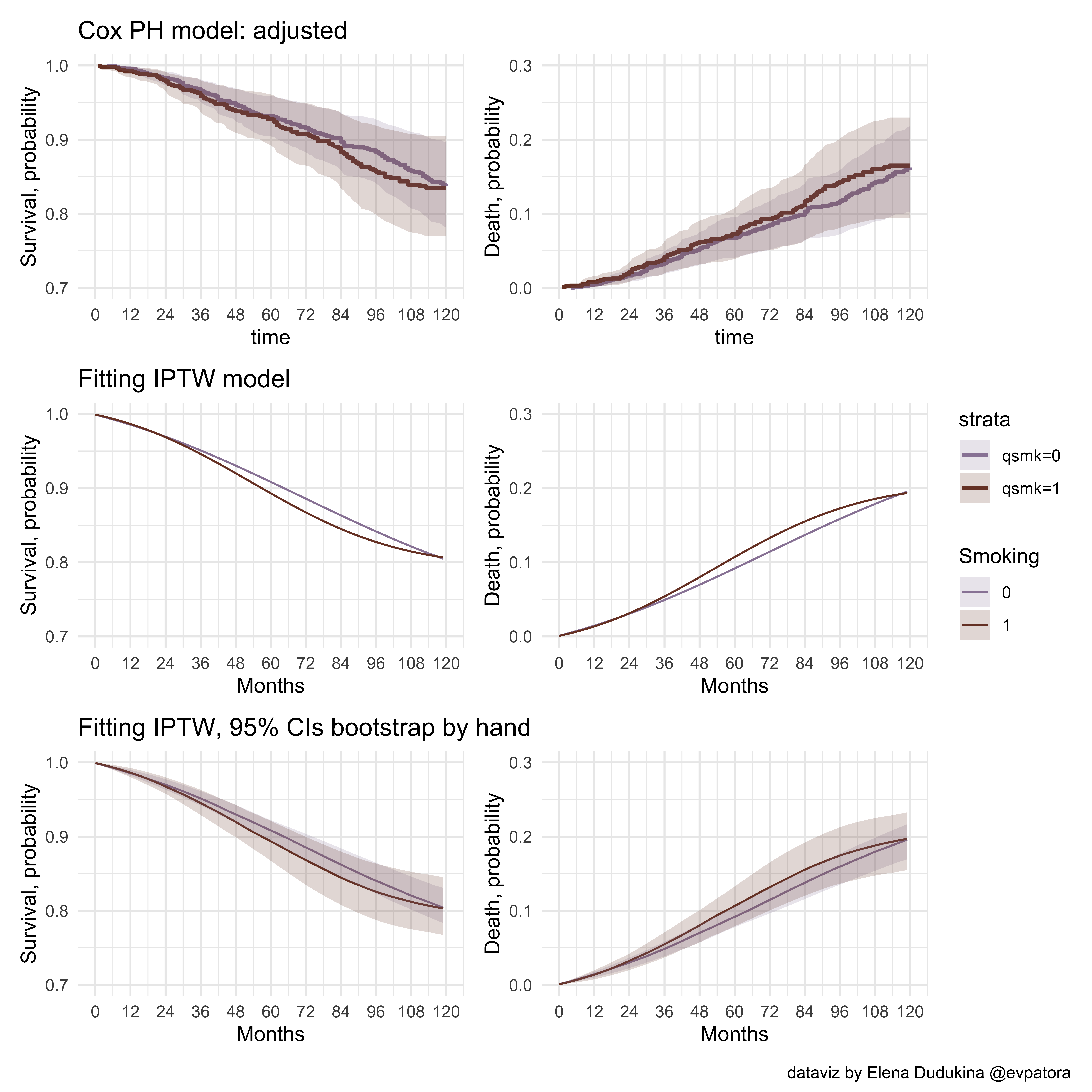
Now I would like to compute and plot 95% confidence intervals for each month data point on the IPTW plot. For this, I’m going to perform bootstrapping “by hand” in the code below. It is not very “pretty” or efficient code, but for me, it gave better understanding of the bootstrapping. For showcasing purposes, I only use 100 bootsraps. To apply the same custom function with the specifications of IPTW model to the list of resampled datasets, I use `purrr::exec' function. Later, I use percentile method to compute 95% CIs for the ATE of smoking on mortality over time. At the time of posting this, there is no equivalent code in currently available chaperon R materials for “What If” Chapter 17.
# keep only needed vars
data_iptw <- months_iptw %>%
dplyr::select(seqn, qsmk, time, timesq, event, iptw_stab)
# bootstrap IPTW model
# IPTW model using GLM as an approximation for the hazard model (no embedded selection bias as in Cox PH model)
boot_n <- 100 # number of bootstraps; for showcasing, I only use 100 bootstraps
sample_n <- nrow(data_iptw) # size of the sample for each bootstrap iteration
# original data to take samples from
data_list <- rep(list(data_iptw), times = boot_n)
set.seed(123456789)
resampled_data_list <- map(data_list, ~ sample_n(., size = sample_n, replace = T)) # resampling with replacement
# the function I want to plug the data list in; this function will be iterated over the list of resampled datasets
iptw_model <- function(data) {
glm(formula = event == 0 ~ qsmk + qsmk*time + qsmk*timesq + time + timesq,
family = binomial(link = "logit"),
weight = iptw_stab,
data = data)
}
# map IPTW modeling function over the list of resampled datasets using purrr::exec
model_fits_list <- map(resampled_data_list, ~exec(iptw_model, .x))
# created the list of the tidy dataset with the modeling results
tidy_fits_list <- map(model_fits_list, ~ broom::tidy(., conf.int = F, exponentiate = T))
# make a large dataset of all results of all iterations
tidy_fits <- tidy_fits_list %>%
bind_rows(.id = "iteration")
tidy_fits_perc <- tidy_fits %>%
group_by(term) %>%
summarise_at(.vars = vars(estimate), .funs = list(Q2.5 = ~ quantile(., probs = 0.025), Q50 = ~ quantile(., probs = 0.50), Q97.5 = ~ quantile(., probs = 0.975)))
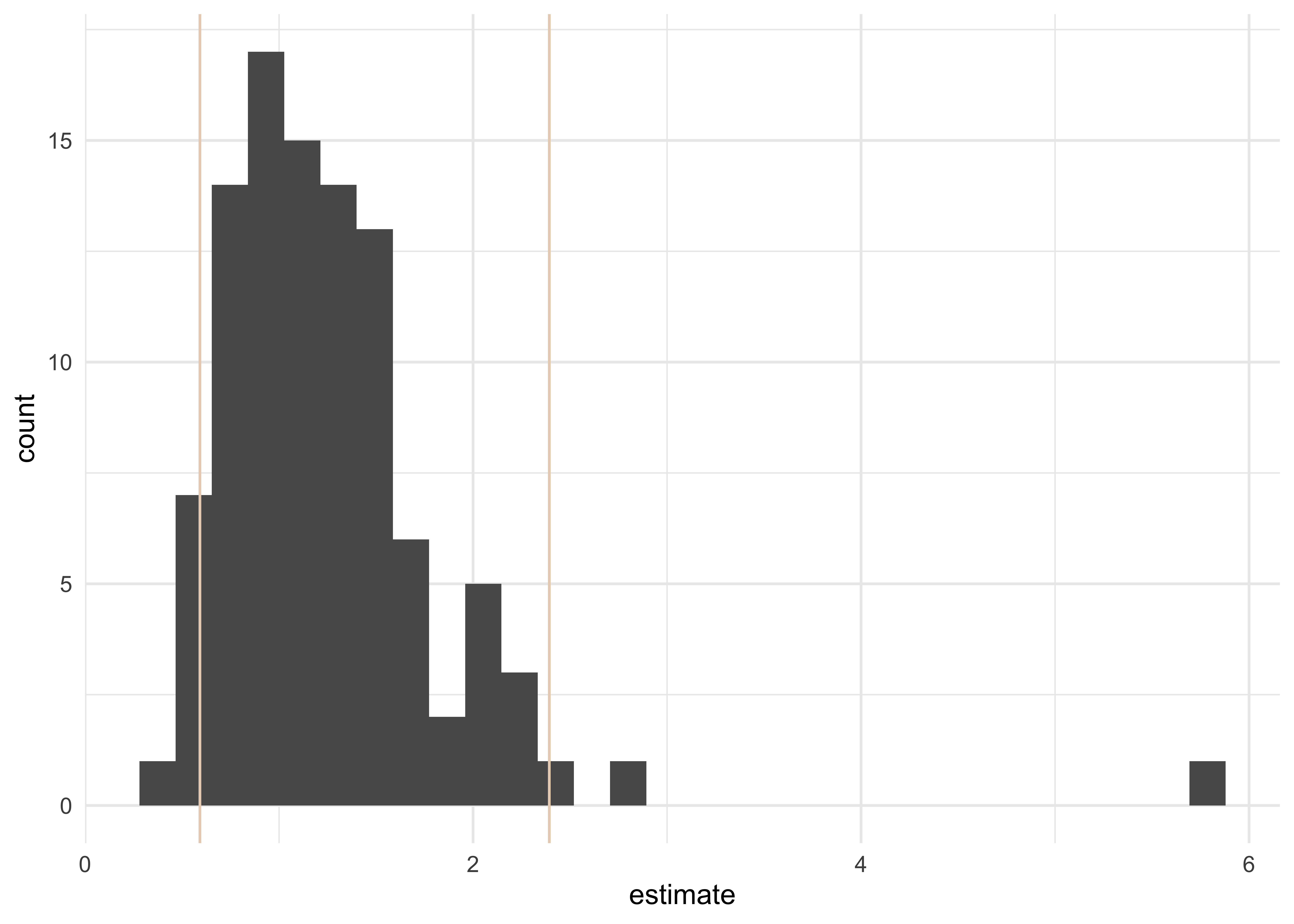
# assess percentile 95% CI graphically
tidy_fits %>%
filter(term == "qsmk") %>%
ggplot(aes(estimate)) +
geom_histogram(bins = 30) +
theme_minimal() +
geom_vline(aes(xintercept = Q2.5), data = tidy_fits_perc %>% filter(term == "qsmk"), col = "#AA9486") +
geom_vline(aes(xintercept = Q97.5), data = tidy_fits_perc %>% filter(term == "qsmk"), col = "#AA9486")
# create the dataset with all observation-months under each treatment level (treated, untreated)
# list: every month with the assigned exposure level = 0
months0_iptw <- tibble(time = seq(0, 119),
                  qsmk = 0,
                  timesq = seq(0, 119)^2)

list_months0_iptw <- rep(list(months0_iptw), times = boot_n)

# list: every month with the assigned exposure level = 1
months1_iptw <- tibble(time = seq(0, 119),
                  qsmk = 1,
                  timesq = seq(0, 119)^2)

list_months1_iptw <- rep(list(months1_iptw), times = boot_n)

# assign estimated 1-"hazard" to each observation-month in each observation-months using the list of IPTW model fitted to resampled datasets; NB: newdata argument
list_months0_iptw %<>%
    map2(.x = ., .y = model_fits_list, ~ mutate(.x,
      p.not.event = predict(.y, type = "response", newdata = .x))
  )

list_months1_iptw %<>%
    map2(.x = ., .y = model_fits_list, ~ mutate(.x,
      p.not.event = predict(.y, type = "response", newdata = .x))
  )

# compute survival for each observation-month
list_months0_iptw %<>%
  map(.x = ., ~mutate(.x,
    # to find a cumulative probability of not-event take a cumulative product of probabilities
    p.surv = cumprod(p.not.event)
  )
)

list_months1_iptw %<>%
  map(.x = ., ~mutate(.x,
    # to find a cumulative probability of not-event take a cumulative product of probabilities
    p.surv = cumprod(p.not.event)
  )
)

# difference in survival in each observation month
surv_diff_iptw_list <- map(list(list_months0_iptw, list_months1_iptw), ~bind_rows(., .id = "iteration"))

surv_diff_iptw <- surv_diff_iptw_list %>% bind_cols(.) %>%
  mutate(
    surv_diff_iptw = p.surv...12 - p.surv...6
  )
## New names:
## * iteration -> iteration...1
## * time -> time...2
## * qsmk -> qsmk...3
## * timesq -> timesq...4
## * p.not.event -> p.not.event...5
## * ...
surv_diff_iptw %<>%
  group_by(time...2) %>%
  summarise_at(.vars = vars(surv_diff_iptw), .funs = list(Q2.5 = ~ quantile(., probs = 0.025), Q50 = ~ quantile(., probs = 0.50), Q97.5 = ~ quantile(., probs = 0.975)))

# bind and plot
surv_diff_iptw_plot <- surv_diff_iptw_list %>% bind_rows(., .id = "id")

# percentile method for 95% CIs
surv_diff_iptw_plot %<>%
  group_by(qsmk, time) %>%
  summarise_at(.vars = vars(p.surv), .funs = list(Q2.5 = ~ quantile(., probs = 0.025), Q50 = ~ quantile(., probs = 0.50), Q97.5 = ~ quantile(., probs = 0.975)))
# survival IPTW with 95% CIs
p2_glm_1 <- surv_diff_iptw_plot %>%
  group_by(qsmk) %>%
  ggplot(aes(x = time, y = Q50, color = factor(qsmk), fill = factor(qsmk))) +
  geom_line() +
  geom_ribbon(aes(ymin = Q2.5, ymax = Q97.5), alpha = .2, colour = NA) +
  scale_x_continuous(limits = c(0, 120), breaks = seq(0, 120, 12)) +
  scale_y_continuous(limits = c(0.7, 1), breaks = seq(0.7, 1, 0.1)) +
  xlab("Months") +
  ylab("Survival, probability") +
  ggtitle("Fitting IPTW, 95% CIs bootstrap by hand") +
  theme_minimal()+
  labs(colour = "Smoking", fill = "Smoking") +
  scale_fill_manual(values = wes_palette("IsleofDogs1")) +
  scale_color_manual(values = wes_palette("IsleofDogs1"))

# 1-survival
p2_glm_2 <- surv_diff_iptw_plot %>%
  group_by(qsmk) %>%
  ggplot(aes(x = time, y = 1 - Q50, color = factor(qsmk), fill = factor(qsmk))) +
  geom_line() +
  geom_ribbon(aes(ymin = 1 - Q97.5, ymax = 1 - Q2.5), alpha = .2, colour = NA) +
  scale_x_continuous(limits = c(0, 120), breaks = seq(0, 120, 12)) +
  scale_y_continuous(limits = c(0, 0.3), breaks = seq(0, 0.3, 0.1)) +
  xlab("Months") +
  ylab("Death, probability") +
  theme_minimal()+
  labs(colour = "Smoking", fill = "Smoking") +
  scale_fill_manual(values = wes_palette("IsleofDogs1")) +
  scale_color_manual(values = wes_palette("IsleofDogs1"))

p2_glm_3 <- surv_diff_iptw %>%
  ggplot(aes(x = time...2, y = Q50)) +
  geom_line() +
  geom_ribbon(aes(ymin = Q2.5, ymax = Q97.5), alpha = .2, colour = NA) +
  scale_x_continuous(limits = c(0, 120), breaks = seq(0, 120, 12)) +
  xlab("Months") +
  ylab("Difference") +
  theme_minimal()+
  labs(colour = "Smoking", fill = "Smoking")

# combine IPTW plots
p2_glm_1 / p2_glm_2 / p2_glm_3 +
  plot_layout(guides = "collect")
# combine all plots
comb2 <- cox_adj_p1 + cox_adj_p2 + p_iptw_1 + p_iptw_2 + p2_glm_1 + p2_glm_2 +
  plot_layout(ncol = 2, guides = "collect") +
  plot_annotation(
  caption = "dataviz by Elena Dudukina @evpatora"
)
comb2
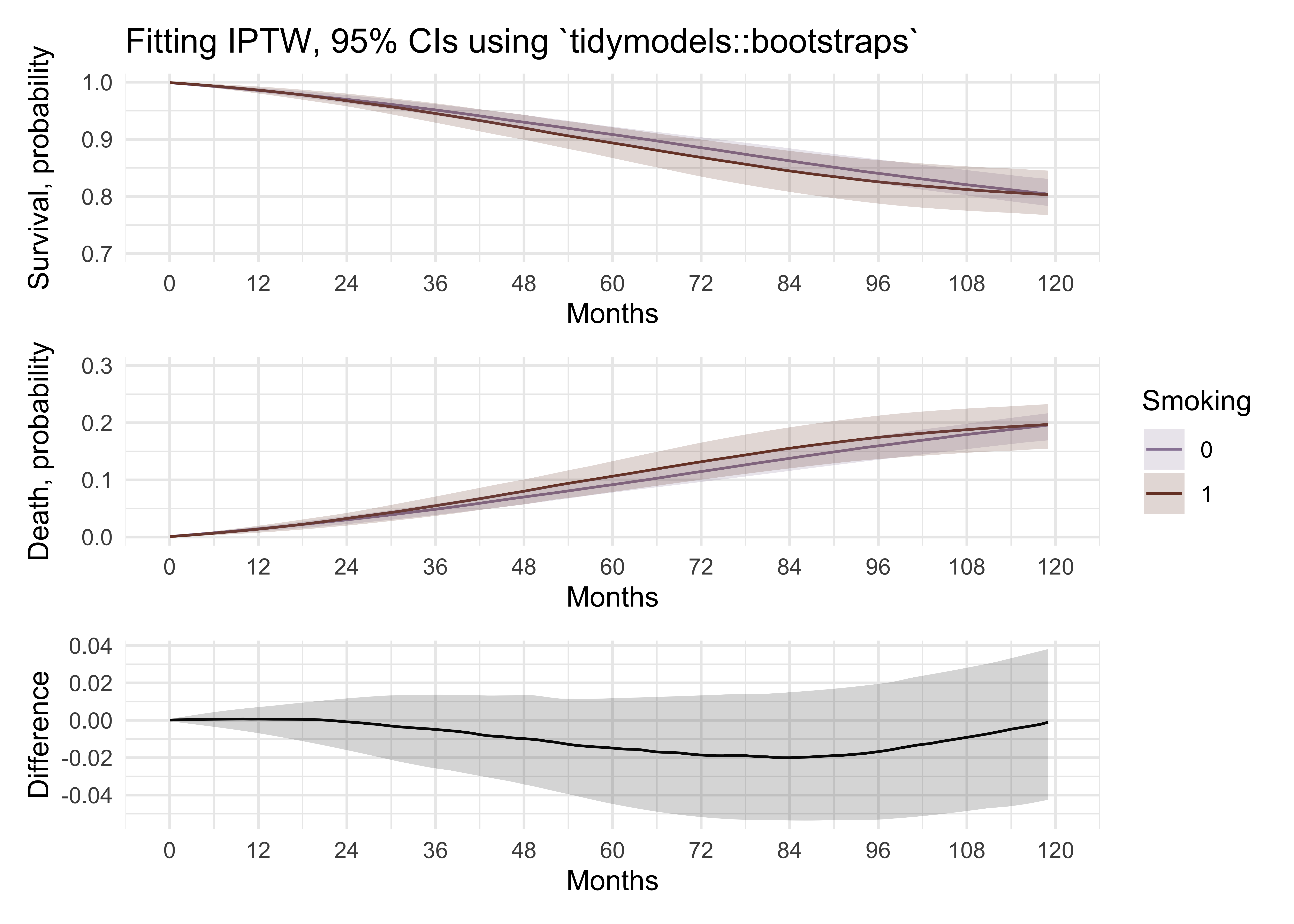
Using tidymodels to perform bootstrapping.
library(tidymodels)
## ── Attaching packages ────────────────────────────────────── tidymodels 0.1.3 ──
## ✓ broom        0.7.6      ✓ rsample      0.1.0
## ✓ dials        0.0.9      ✓ tune         0.1.5
## ✓ infer        0.5.4      ✓ workflows    0.2.2
## ✓ modeldata    0.1.0      ✓ workflowsets 0.0.2
## ✓ parsnip      0.1.5      ✓ yardstick    0.0.8
## ✓ recipes      0.1.16
## ── Conflicts ───────────────────────────────────────── tidymodels_conflicts() ──
## x scales::discard()       masks purrr::discard()
## x magrittr::extract()     masks tidyr::extract()
## x dplyr::filter()         masks stats::filter()
## x recipes::fixed()        masks stringr::fixed()
## x dplyr::lag()            masks stats::lag()
## x rsample::permutations() masks gtools::permutations()
## x MASS::select()          masks dplyr::select()
## x magrittr::set_names()   masks purrr::set_names()
## x yardstick::spec()       masks readr::spec()
## x recipes::step()         masks stats::step()
## • Use tidymodels_prefer() to resolve common conflicts.
times <- 100
set.seed(123456789)
boots <- bootstraps(data_iptw, times = times, apparent = FALSE)

# the same IPTW model we've used before
iptw_model <- function(data) {
  glm(formula = event == 0 ~ qsmk + qsmk*time + qsmk*timesq + time + timesq,
                 family = binomial(link = "logit"),
                 weight = iptw_stab,
                 data = data)
}

boot_models <- boots %>%
  mutate(
    model = map(.x = splits, ~iptw_model(data = .x)),
    coef_info = map(model, ~broom::tidy(.x, exponentiate = T)))

boot_coefs <- boot_models %>%
  unnest(coef_info)

percentile_intervals <- int_pctl(boot_models, coef_info)
percentile_intervals
## # A tibble: 6 x 6
##   term         .lower .estimate   .upper .alpha .method
##   <chr>         <dbl>     <dbl>    <dbl>  <dbl> <chr>
## 1 (Intercept) 773.     1054.    1536.      0.05 percentile
## 2 qsmk          0.592     1.27     2.39    0.05 percentile
## 3 qsmk:time     0.953     0.983    1.01    0.05 percentile
## 4 qsmk:timesq   1.00      1.00     1.00    0.05 percentile
## 5 time          0.967     0.980    0.993   0.05 percentile
## 6 timesq        1.00      1.00     1.00    0.05 percentile
# assess percentile 95% CI graphically
boot_coefs %>%
  filter(term == "qsmk") %>%
  ggplot(aes(estimate)) +
  geom_histogram(bins = 30) +
  theme_minimal() +
  geom_vline(aes(xintercept = .lower), data = percentile_intervals %>% filter(term == "qsmk"), col = "#EAD3BF") +
  geom_vline(aes(xintercept = .upper), data = percentile_intervals %>% filter(term == "qsmk"), col = "#EAD3BF")
# observation-month data
months0_iptw <- tibble(time = seq(0, 119),
                  qsmk = 0,
                  timesq = seq(0, 119)^2)

list_months0_iptw <- rep(list(months0_iptw), times = times)

# list: every month with the assigned exposure level = 1
months1_iptw <- tibble(time = seq(0, 119),
                  qsmk = 1,
                  timesq = seq(0, 119)^2)

list_months1_iptw <- rep(list(months1_iptw), times = times)

# assign estimated 1-"hazard" to each observation-month in each observation-months using the list of IPTW model fitted to resampled datasets; NB: newdata argument
list_months0_iptw %<>%
    map2(.x = ., .y = boot_models$model, ~ mutate(.x,
      p.not.event = predict(.y, type = "response", newdata = .x))
  )

list_months1_iptw %<>%
    map2(.x = ., .y = boot_models$model, ~ mutate(.x,
      p.not.event = predict(.y, type = "response", newdata = .x))
  )

# compute survival for each observation-month
list_months0_iptw %<>%
  map(.x = ., ~mutate(.x,
    # to find a cumulative probability of not-event take a cumulative product of probabilities
    p.surv = cumprod(p.not.event)
  )
)

list_months1_iptw %<>%
  map(.x = ., ~mutate(.x,
    # to find a cumulative probability of not-event take a cumulative product of probabilities
    p.surv = cumprod(p.not.event)
  )
)

# difference in survival in each observation month
surv_diff_iptw_list <- map(list(list_months0_iptw, list_months1_iptw), ~bind_rows(., .id = "iteration"))

surv_diff_iptw <- surv_diff_iptw_list %>% bind_cols(.) %>%
  mutate(
    surv_diff_iptw = p.surv...12 - p.surv...6
  )
## New names:
## * iteration -> iteration...1
## * time -> time...2
## * qsmk -> qsmk...3
## * timesq -> timesq...4
## * p.not.event -> p.not.event...5
## * ...
surv_diff_iptw %<>%
  group_by(time...2) %>%
  summarise_at(.vars = vars(surv_diff_iptw), .funs = list(Q2.5 = ~ quantile(., probs = 0.025), Q50 = ~ quantile(., probs = 0.50), Q97.5 = ~ quantile(., probs = 0.975)))

# bind and plot
surv_diff_iptw_plot <- surv_diff_iptw_list %>% bind_rows(., .id = "id")

# percentile method for 95% CIs
surv_diff_iptw_plot %<>%
  group_by(qsmk, time) %>%
  summarise_at(.vars = vars(p.surv), .funs = list(Q2.5 = ~ quantile(., probs = 0.025), Q50 = ~ quantile(., probs = 0.50), Q97.5 = ~ quantile(., probs = 0.975)))
# survival IPTW with 95% CIs
p2_glm_1_tidymodels <- surv_diff_iptw_plot %>%
  group_by(qsmk) %>%
  ggplot(aes(x = time, y = Q50, color = factor(qsmk), fill = factor(qsmk))) +
  geom_line() +
  geom_ribbon(aes(ymin = Q2.5, ymax = Q97.5), alpha = .2, colour = NA) +
  xlab("Months") +
  scale_x_continuous(limits = c(0, 120), breaks = seq(0, 120, 12)) +
  scale_y_continuous(limits = c(0.7, 1), breaks = seq(0.7, 1, 0.1)) +
  ylab("Survival, probability") +
  ggtitle("Fitting IPTW, 95% CIs using `tidymodels::bootstraps`") +
  theme_minimal()+
  labs(colour = "Smoking", fill = "Smoking") +
  scale_fill_manual(values = wes_palette("IsleofDogs1")) +
  scale_color_manual(values = wes_palette("IsleofDogs1"))

# 1-survival
p2_glm_2_tidymodels <- surv_diff_iptw_plot %>%
  group_by(qsmk) %>%
  ggplot(aes(x = time, y = 1 - Q50, color = factor(qsmk), fill = factor(qsmk))) +
  geom_line() +
  geom_ribbon(aes(ymin = 1 - Q97.5, ymax = 1 - Q2.5), alpha = .2, colour = NA) +
  scale_x_continuous(limits = c(0, 120), breaks = seq(0, 120, 12)) +
  scale_y_continuous(limits = c(0, 0.3), breaks = seq(0, 0.3, 0.1)) +
  xlab("Months") +
  ylab("Death, probability") +
  theme_minimal()+
  labs(colour = "Smoking", fill = "Smoking") +
  scale_fill_manual(values = wes_palette("IsleofDogs1")) +
  scale_color_manual(values = wes_palette("IsleofDogs1"))

p2_glm_3_tidymodels <- surv_diff_iptw %>%
  ggplot(aes(x = time...2, y = Q50)) +
  geom_line() +
  geom_ribbon(aes(ymin = Q2.5, ymax = Q97.5), alpha = .2, colour = NA) +
  scale_x_continuous(limits = c(0, 120), breaks = seq(0, 120, 12)) +
  xlab("Months") +
  ylab("Difference") +
  theme_minimal()+
  labs(colour = "Smoking", fill = "Smoking")

# combine IPTW plots
p2_glm_1_tidymodels / p2_glm_2_tidymodels / p2_glm_3_tidymodels +
  plot_layout(guides = "collect")
# combine all plots
comb2 <- cox_adj_p1 + cox_adj_p2 + p_iptw_1 + p_iptw_2 + p2_glm_1 + p2_glm_2 + p2_glm_1_tidymodels + p2_glm_2_tidymodels +
  plot_layout(ncol = 2, guides = "collect") +
  plot_annotation(
  caption = "dataviz by Elena Dudukina @evpatora"
)
comb2
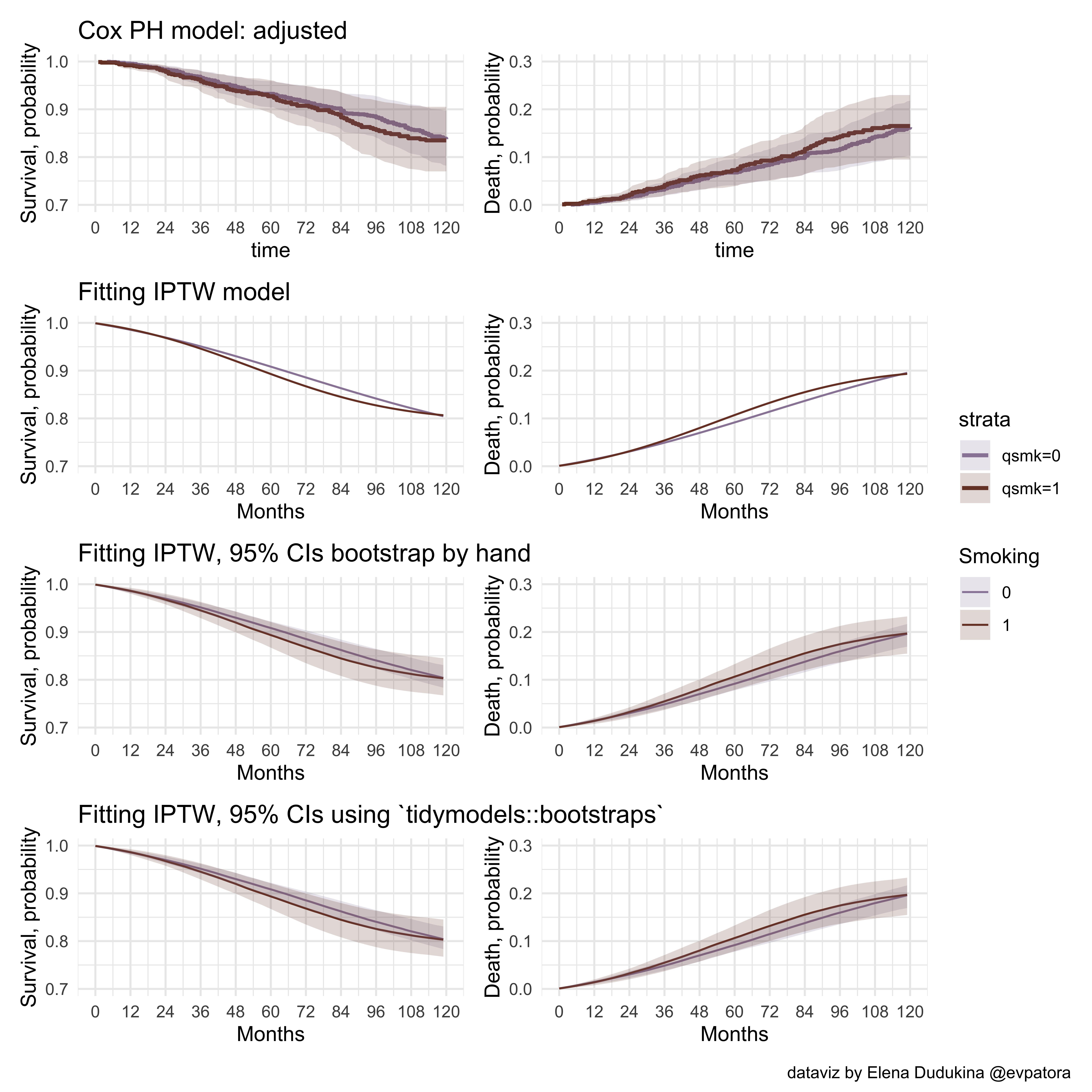
My “by hand” bootstrapping gave the same results as bootstrapping with tidymodels. Phew 😄
Final notes
When interpreting the results of model fitting with IPTW do not forget to return to your
- Causal question
- Causal diagram (DAG)
- Causal assumptions
References
- Hernán MA, Robins JM (2020). Causal Inference: What If. Boca Raton: Chapman & Hall/CRC
- R code by Joy Shi and Sean McGrath available here
Additional info
- Dr Ellie Murray’s tweetorials
The results of my #tweetorial poll were pretty clear: from over 350 votes, 38% of you want to know about causal survival analysis. So, pull up a chair and let’s talk time-to-event! pic.twitter.com/nAtyxQAnWU
— Dr Ellie Murray (@EpiEllie) November 11, 2018
Interested in estimating causal effects on survival outcomes? You may need to account for time-varying confounders. Don’t know how?
— Dr Ellie Murray (@EpiEllie) October 11, 2020
My new paper with @elliecaniglia & @lucia_petito explains the basics, with #Rstats, SAS, & stata code!#causaltwitter https://t.co/4HIERDE5hd