Competing events survival analyses
This is an account of R code by Paloma Rojas-Saunero, PhD available
here, which I “translated” to tidyverse code and added some clarifications and figures. This is a longer read, but, hopefully, also is easier to follow for those who use tidyverse.
Rationale
Competing events in survival analyses are hard to implement and available estimators may lack truly causal interpretation under potential outcomes/counterfactual framework.
Code implementation
Without these functions, the example will not work.
# NB! VERY IMPORTANT
# getting the utility functions from [Young et al. Statistics in Medicine. 2020](https://onlinelibrary.wiley.com/doi/abs/10.1002/sim.8471) supplement R code "pgform_ipwcs.R"
# These functions are copy-pasted from the cited file without any modifications

# utility functions for IPW estimators
nonParametricCumHaz <- function(weightVector, inputdata, grp, outcomeProstate=TRUE){
  outputHazards <- rep(NA, length.out=length(cutTimes))
  counter <- 1
  for(i in cutTimes){
    if(outcomeProstate){
      indices <- inputdata$dtime==i & inputdata$rx == grp & inputdata$eventCens==0 & inputdata$otherDeath==0
      eventIndicator <- indices & inputdata$prostateDeath==1
    }else{
      indices <- inputdata$dtime==i & inputdata$rx == grp & inputdata$eventCens==0
      eventIndicator <- indices & inputdata$otherDeath==1
    }
    outputHazards[counter] <- sum(weightVector[eventIndicator]) / sum(weightVector[indices])
    counter <- counter+1
  }
  return(outputHazards)
}

nonParametricCumInc <- function(hazard1,hazard2,competing=FALSE){
  inc <- rep(NA, length.out=length(cutTimes))
  cumulativeSurvival <- c(1, cumprod( (1-hazard1) * (1-hazard2) ))
  counter <- 1
  for(i in 1:length(cutTimes)){
    if(!competing){
      inc[i] <- hazard1[i] * (1-hazard2[i]) * cumulativeSurvival[i]
    }else{
      inc[i] <- hazard1[i] * cumulativeSurvival[i]
    }
  }
  cumInc <- cumsum(inc)
  return(cumInc)
}

# Utility function for parametric g-formula estimators (for separable effects section)
# NB!!!!! keep note of the variables and objects' names in the function!
# NB!!!!! updated the function to allow hazardP and hazardO have user-flexible names
# non-flexible parameters in the function:
# var name patno is per specific example dataset
# variable s for creating survivalProb

calculateCumInc <- function(inputData,timepts=cutTimes,hazardO="hazardO",hazardP="hazardP",competing=FALSE){
  cumulativeIncidence <- matrix(NA,ncol = length(unique(inputData$patno)),nrow = length(timepts))
  # Insert the event probabilities at the first time interval:
  # Needs to account for "temporal order" Dk+1 before Yk+1
  if(!competing) cumulativeIncidence[1,] <- inputData[inputData$dtime==0,][[hazardP]]*(1-inputData[inputData$dtime==0,][[hazardO]])
  else cumulativeIncidence[1,] <- inputData[inputData$dtime==0,][[hazardO]]
  # Create a matrix compatible with 'cumulativeIncidence' with survival probabilities at each time
  survivalProb <- t(aggregate(s~patno,data = inputData, FUN = cumprod)$s) #split the long data into subsets per subject
  for(i in 2:length(timepts)){
    subInputDataP <- inputData[inputData$dtime==(i-1),][[hazardP]]#OBS: dtime starts at 0
    subInputDataO <- inputData[inputData$dtime==(i-1),][[hazardO]] #OBS: dtime starts at 0
    if(!competing) cumulativeIncidence[i,] <- subInputDataP * (1-subInputDataO) *  survivalProb[(i-1),] # OBS: survivalProb entry i is time point i-1
    else cumulativeIncidence[i,] <- subInputDataO * survivalProb[(i-1),]
  }
  meanCumulativeIncidence <- rowMeans(apply(cumulativeIncidence, MARGIN = 2,cumsum))
  return(meanCumulativeIncidence)
}
Reshaping prostate cancer dataset for pooled logistic regression over follow-up time
Getting the data: Byar & Greene’s dataset.
data <- read.csv(paste0(path, "prostate.csv"), sep = ';')
Create an indicator for all-cause mortality: 0=alive, 1=dead
data %<>% mutate(
  allCause = if_else(status != "alive", 1, 0)
)
Create a variable with 3 levels (a level for each cause of death)
data %<>% mutate(
  eventType = case_when(
    status == "alive" ~ "alive",
    status == "dead - prostatic ca" ~ "pdeath",
    T ~ "odeath"
  ),
  # set factor levels
  eventType = factor(eventType, levels = c("alive", "pdeath", "odeath"))
)
Create comparator groups: A=1 (high dose DES) and A=0 (placebo)
data %<>%
  mutate(
  rx = as_factor(rx)
) %>%
  filter(rx %in% c("placebo", "5.0 mg estrogen")) %>%
  mutate(
    temprx = as.integer(rx) - 2,
    rx = abs(1 - temprx), # DES: A=1 and placebo: A=0
    eventType = as.integer(eventType) - 1, #0: censoring, 1: pdeath, 2: odeath
    hgBinary = if_else(hg < 12, 1, 0),
    ageCat = Hmisc::cut2(age, c(0, 60, 70, 80, 100)),
    normalAct = if_else(pf == "normal activity", 1, 0),
    eventCens = if_else(eventType == 0, 1, 0),
    eventProst = if_else(eventType == 1, 1, 0),
    Tstart = -0.01 # for long format transformation later
  )
Mortality risk at the end of data by rx status (high dose DES vs placebo)
data %>% select(rx, eventType) %>%
  mutate(rx = case_when(rx == 0 ~ "Placebo", T ~ "High dose DES"),
         eventType = case_when(eventType == 0 ~ "Alive",
                               eventType == 1 ~ "Prostate cancer death",
                               T ~ "Other cause of death")) %>%
  gtsummary::tbl_summary(by = rx) %>%
  gtsummary::modify_header(label = "**Variable**") %>% # update the column header
  gtsummary::bold_labels()
| Variable | High dose DES, N = 1251 | Placebo, N = 1271 |
|---|---|---|
| eventType | ||
| Alive | 32 (26%) | 32 (25%) |
| Other cause of death | 66 (53%) | 58 (46%) |
| Prostate cancer death | 27 (22%) | 37 (29%) |
| 1 n (%) | ||
Create long format dataset
cutTimes <- c(0:59)

data_prost_cens_long <- data %>%
  survSplit(
    cut = cutTimes,
    start = "Tstart",
    end = "dtime",
    event = "eventCens")

data_prost_long <- data %>%
  survSplit(
    cut = cutTimes,
    start = "Tstart",
    end = "dtime",
    event = "allCause") %>%
  mutate(
    eventCens = data_prost_cens_long$eventCens,
    # prostate cancer mortality indicator
    prostateDeath = if_else(allCause == 1 & eventType == 1, 1, 0),
    # other causes of death indicator
    otherDeath = if_else(allCause == 1 & eventType == 2, 1, 0)
  )
Do not condition on “future data” by setting prostate cancer death or death from other causes to missing in every observation after it has been censored; set prostate cancer death to missing after an death from other causes was observed.
data_prost_long %<>% mutate(
  # unless censored or died from other than prostate cancer causes - the outcome is defined, otherwise - undefined
  prostateDeath = if_else(eventCens == 1, NA_real_, prostateDeath),
  otherDeath = if_else(eventCens == 1, NA_real_, otherDeath),
  prostateDeath = if_else(otherDeath == 1, NA_real_, prostateDeath)
)
For fitting pooled over time logistic regression models, only keep observations with \(dtime < K + 1\)
data_prost_long %<>% filter(dtime < length(cutTimes))
Create T0 data: data at time point 0
T0 <- data_prost_long %>% filter(dtime == 0)

# number of individuals at baseline
n <- n_distinct(data_prost_long$patno)
Computation of IPT weights
A set of conditional pooled logistic regression models for constructing IPCW. First, a set of models for the denominators for each potential end of data: prostate cancer death, death due to other causes, censoring. The estimated parameter: probability of death/censoring given exposure and potential confounding factors.
# Model for prostate cancer death
pdeath_fit <-
  glm(prostateDeath ~ rx * (dtime + I(dtime ^ 2) + I(dtime ^ 3)) + normalAct + ageCat + hx + hgBinary ,
    data = data_prost_long,
    family = binomial(link = "logit")
    )

# Model for mortality from other causes
odeath_fit <-
  glm(otherDeath ~ dtime + I(dtime ^ 2) + normalAct + ageCat + hx + hgBinary + rx ,
    data = data_prost_long,
    family = binomial(link = "logit")
    )

# keep data for dtime > 50
cens50 <- data_prost_long %>% filter(dtime > 50)

# Model for censoring
pcens_fit <-
  glm(eventCens ~  normalAct + ageCat + hx + rx,
      data = cens50,
      family = binomial(link = "logit")
      )
Second, a set of models to construct numerators for stabilized IPCW. The estimated parameter is the probability of censoring/other death given the exposure level.
cens_num_fit <- glm(eventCens ~ rx , data = cens50, family = binomial(link = "logit"))

odeath_num_fit <- glm(otherDeath ~ dtime + I(dtime ^ 2) + rx,
      data = data_prost_long,
      family = binomial(link = "logit"))
Compute unstabilized and stabilized inverse probability of censoring weights (IPCW) due to loss-to-follow-up
data_prost_long %<>% mutate(
  # predicted probability of censoring: denominator
  pred_c = case_when(
    dtime > 50 ~ 1 - predict(pcens_fit, ., type = "response"),
    T ~ 1
  ),
  # predicted probability of censoring: numerator
  pred_c_num = case_when(
    dtime > 50 ~ 1 - predict(cens_num_fit, ., type = "response"),
    T ~ 1
  )
) %>%
  group_by(patno) %>%
  mutate(
    # cumulative product per patient over all months
  cum_pred_c = cumprod(pred_c),
  cum_pred_c_num = cumprod(pred_c_num)
  ) %>%
  ungroup() %>%
  mutate(
    ipcw_cens_unstab = 1/cum_pred_c,
    ipcw_cens_stab = cum_pred_c_num/cum_pred_c
  )
Compute IPCWs for other than prostate cancer death as competing event
data_prost_long %<>% mutate(
pred_odeath = 1 - predict(odeath_fit, newdata = ., type = 'response'),
pred_odeath_num = 1 - predict(odeath_num_fit, newdata = ., type = 'response')
) %>%
group_by(patno) %>%
#cumulative probability of other death per person over all months
mutate(
cum_pred_odeath = cumprod(pred_odeath),
cum_pred_odeath_num = cumprod(pred_odeath_num)
) %>%
ungroup() %>%
mutate(
ipcw_odeath_unstab = 1/cum_pred_odeath,
ipcw_odeath_stab = cum_pred_odeath_num/cum_pred_odeath,
# combined weights for censoring due to the loss-of-follow-up and other than prostate cancer death (Censoring or Other Death)
ipcw_cod_unstab = ipcw_cens_unstab * ipcw_odeath_unstab,
ipcw_cod_stab = ipcw_cens_stab * ipcw_odeath_stab
)
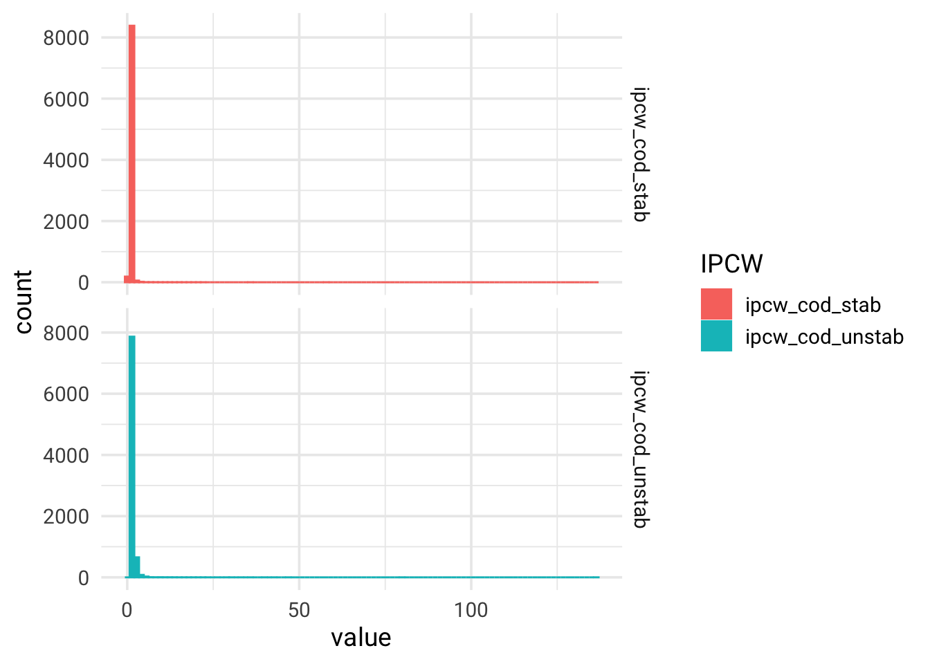
# quick summary of the weights
summary(data_prost_long$ipcw_cod_unstab)
##    Min. 1st Qu.  Median    Mean 3rd Qu.    Max.
##   1.003   1.111   1.260   1.518   1.532 136.741
summary(data_prost_long$ipcw_cod_stab)
##    Min. 1st Qu.  Median    Mean 3rd Qu.    Max.
##  0.3996  0.8531  0.9681  1.0335  1.0750 57.9902
# NB! some unstabilized weights are above 100

data_prost_long %>%
  pivot_longer(cols = c(ipcw_cod_stab, ipcw_cod_unstab), names_to = "IPCW", values_to = "value") %>%
  ggplot(aes(x = value, color = IPCW, fill = IPCW)) +
    geom_histogram(bins = 100) +
    facet_grid(rows = vars(IPCW)) +
  theme_minimal(base_size = 14, base_family = "Roboto")
Computing direct effect
Direct effect refers to the causal effect of high dose DES therapy vs untreated on prostate cancer mortality not mediated via death from other causes (equation (37), Young et al. Statistics in Medicine. 2020) using weighted Kaplan-Meier estimator (“IPW estimator can be constructed as the complement of a weighted product-limit (Kaplan-Meier) estimator”).
Cumulative hazard and cumulative incidence for each treatment regime
# Cumulative hazard and cumulative incidence for the high dose DES: A=1

#### Unstabilized
hazard_treated_ipcw_cod_unstab <- nonParametricCumHaz(data_prost_long$ipcw_cod_unstab,
                                                      inputdata = data_prost_long, grp = 1,
                                                      outcomeProstate = TRUE)

hazardO_treated_ipcw_cod_unstab <- rep(0, length.out = (length(cutTimes)))

cuminc_treated_ipcw_cod_unstab <- nonParametricCumInc(hazard1 = hazard_treated_ipcw_cod_unstab,
                                                      hazardO_treated_ipcw_cod_unstab)

ipcw_unstab_data_treated <- bind_cols("hazard_treated" = hazard_treated_ipcw_cod_unstab,
                                      "hazardO_treated" = hazardO_treated_ipcw_cod_unstab,
                                      "cuminc_treated" = cuminc_treated_ipcw_cod_unstab)

#### Stabilized
hazard_treated_ipcw_cod_stab <- nonParametricCumHaz(data_prost_long$ipcw_cod_stab,
                                                    inputdata = data_prost_long, grp = 1,
                                                    outcomeProstate = TRUE)

hazardO_treated_ipcw_cod_stab <- rep(0, length.out = (length(cutTimes)))

cuminc_treated_ipcw_cod_stab <- nonParametricCumInc(hazard1 = hazard_treated_ipcw_cod_stab,
                                                    hazardO_treated_ipcw_cod_stab)

ipcw_stab_data_treated <- bind_cols("hazard_treated" = hazard_treated_ipcw_cod_stab,
                                    "hazardO_treated" = hazardO_treated_ipcw_cod_stab,
                                    "cuminc_treated" = cuminc_treated_ipcw_cod_stab)

# checking that the data sets are not identical
identical(ipcw_unstab_data_treated, ipcw_stab_data_treated)
## [1] FALSE
### Calculate cumulative hazard and cumulative incidence for the untreated: A=0

#### Unstabilized
hazard_untreated_ipcw_cod_unstab <- nonParametricCumHaz(data_prost_long$ipcw_cod_unstab,
                                                        inputdata = data_prost_long, grp = 0,
                                                        outcomeProstate = TRUE)

hazardO_untreated_ipcw_cod_unstab <- rep(0, length.out = (length(cutTimes)))

cuminc_untreated_ipcw_cod_unstab <- nonParametricCumInc(hazard1 = hazard_untreated_ipcw_cod_unstab,
                                                        hazardO_untreated_ipcw_cod_unstab)

ipcw_unstab_data <- bind_cols("hazard_untreated" = hazard_untreated_ipcw_cod_unstab,
                              "hazardO_untreated" = hazardO_untreated_ipcw_cod_unstab,
                              "cuminc_untreated" = cuminc_untreated_ipcw_cod_unstab) %>%
  bind_cols(ipcw_unstab_data_treated)

#### Stabilized
hazard_untreated_ipcw_cod_stab <- nonParametricCumHaz(data_prost_long$ipcw_cod_stab,
                                                      inputdata = data_prost_long, grp = 0,
                                                      outcomeProstate = TRUE)

hazardO_untreated_ipcw_cod_stab <- rep(0, length.out = (length(cutTimes)))

cuminc_untreated_ipcw_cod_stab <- nonParametricCumInc(hazard1 = hazard_untreated_ipcw_cod_stab,
                                                      hazardO_untreated_ipcw_cod_stab)

ipcw_stab_data <- bind_cols("hazard_untreated" = hazard_untreated_ipcw_cod_stab,
                            "hazardO_untreated" = hazardO_untreated_ipcw_cod_stab,
                            "cuminc_untreated" = cuminc_untreated_ipcw_cod_stab) %>%
  bind_cols(ipcw_stab_data_treated)
Computing risks, risk difference and risk ratio at 60 months of follow-up for high dose DES vs no treatment on mortality from prostate cancer when deaths from other causes were eliminated (direct effect).
direct_effect <- list("IPCW, unstabilized" = ipcw_unstab_data, "IPCW, stabilized" = ipcw_stab_data) %>%
  map(~mutate(.x,
    RR = cuminc_treated_ipcw_cod_unstab/cuminc_untreated_ipcw_cod_unstab,
    RD = cuminc_treated_ipcw_cod_unstab - cuminc_untreated_ipcw_cod_unstab
  )) %>%
  bind_rows(.id = "IPCW type")

direct_effect %>%
  select(`IPCW type`, cuminc_treated, cuminc_untreated, RR, RD) %>%
  group_by(`IPCW type`) %>%
  filter(
    row_number() == 60
  ) %>%
  mutate_all(., ~round(., 2)) %>%
  ungroup() %>%
  knitr::kable()
## `mutate_all()` ignored the following grouping variables:
## • Column `IPCW type`
## ℹ Use `mutate_at(df, vars(-group_cols()), myoperation)` to silence the message.
| IPCW type | cuminc_treated | cuminc_untreated | RR | RD |
|---|---|---|---|---|
| IPCW, unstabilized | 0.35 | 0.37 | 0.95 | -0.02 |
| IPCW, stabilized | 0.35 | 0.37 | 0.95 | -0.02 |
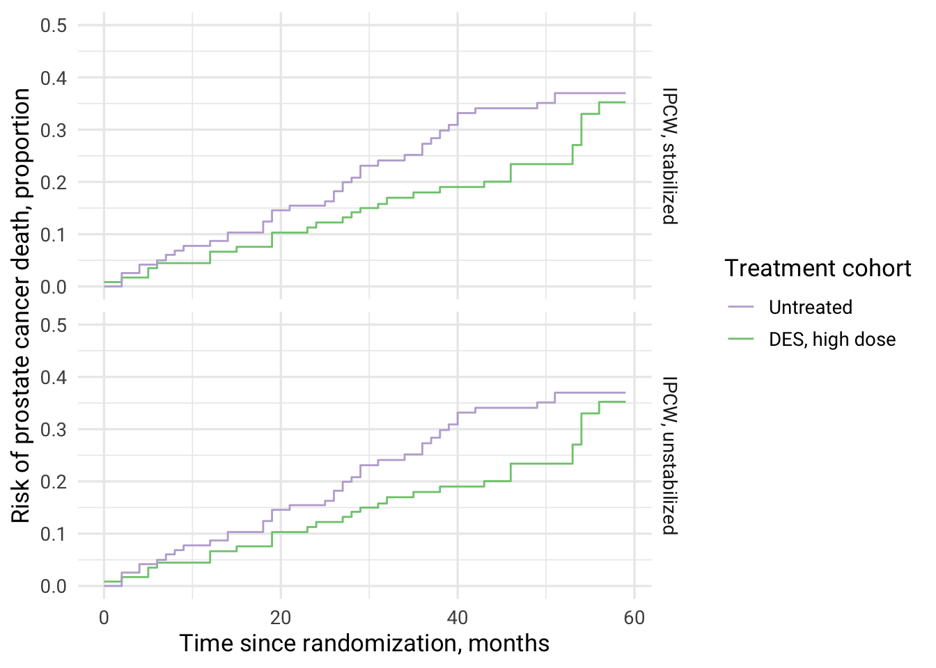
Creating IPC-weighted survival curves for computed direct effect using ggplot2.
direct_effect %>%
  select(`IPCW type`, cuminc_untreated, cuminc_treated) %>%
  group_by(`IPCW type`) %>%
  mutate(
    time = row_number() - 1
  ) %>%
  ungroup() %>%
  pivot_longer(
    cols = c(cuminc_untreated, cuminc_treated),
    names_to = c("cohort"),
    values_to = "cuminc_value"
  ) %>%
  ggplot(aes(x = time, y = cuminc_value, color = cohort, fill = cohort)) +
  geom_step(stat = "identity") +
  scale_y_continuous(limits = c(0,0.5)) +
  theme_minimal(base_size = 13, base_family = "Roboto") +
  scale_color_brewer(palette = "Accent", breaks=c("cuminc_untreated", "cuminc_treated"),
                     labels=c("Untreated", "DES, high dose"), guide = guide_legend(reverse=F)) +
  xlab("Time since randomization, months") +
  ylab("Risk of prostate cancer death, proportion") +
  labs(color = "Treatment cohort") +
  facet_grid(rows = vars(`IPCW type`))
Computing total effect
Total effect refers to the causal effect of high dose DES therapy vs untreated on prostate cancer mortality (cause-specific model) mediated via death from other causes (equation (40)) and taking into account loss to follow-up Young et al. Statistics in Medicine. 2020), i.e. this is “IPW estimator based on weighted estimates of the observed cause-specific hazards of the event of interest and the competing event”. This estimator “coincides with a weighted Aalen-Johansen estimator”. In this scenario, competing events are not eliminated.
# Cumulative hazards and cumulative incidence for the high dose DES: A=1

#### Unstabilized
hazard_treated_ipcw_cens_unstab <- nonParametricCumHaz(data_prost_long$ipcw_cens_unstab,
                                                       inputdata = data_prost_long, grp = 1,
                                                       outcomeProstate = TRUE)

hazardO_treated_ipcw_cens_unstab <- nonParametricCumHaz(data_prost_long$ipcw_cens_unstab,
                                                        inputdata = data_prost_long, grp = 1,
                                                        outcomeProstate = FALSE)

cuminc_treated_ipcw_cens_unstab <- nonParametricCumInc(hazard1 = hazard_treated_ipcw_cens_unstab,
                                                       hazardO_treated_ipcw_cens_unstab)

ipcw_unstab_data_treated <- bind_cols("hazard_treated" = hazard_treated_ipcw_cens_unstab,
                                      "hazardO_treated" = hazardO_treated_ipcw_cens_unstab,
                                      "cuminc_treated" = cuminc_treated_ipcw_cens_unstab)

#### Stabilized
hazard_treated_ipcw_cens_stab <- nonParametricCumHaz(data_prost_long$ipcw_cens_stab,
                                                     inputdata = data_prost_long, grp = 1,
                                                     outcomeProstate = TRUE)

hazardO_treated_ipcw_cens_stab <- nonParametricCumHaz(data_prost_long$ipcw_cens_stab,
                                                      inputdata = data_prost_long, grp = 1,
                                                      outcomeProstate = FALSE)

cuminc_treated_ipcw_cens_stab <- nonParametricCumInc(hazard1 = hazard_treated_ipcw_cens_stab,
                                                     hazardO_treated_ipcw_cens_stab)

ipcw_stab_data_treated <- bind_cols("hazard_treated" = hazard_treated_ipcw_cens_stab,
                                    "hazardO_treated" = hazardO_treated_ipcw_cens_stab,
                                    "cuminc_treated" = cuminc_treated_ipcw_cens_stab)

# checking that the data sets are not identical
identical(ipcw_unstab_data_treated, ipcw_stab_data_treated)
## [1] FALSE
### Calculate cumulative hazards and cumulative incidence for the untreated: A=0

#### Unstabilized
hazard_untreated_ipcw_cens_unstab <- nonParametricCumHaz(data_prost_long$ipcw_cens_unstab,
                                                         inputdata = data_prost_long, grp = 0,
                                                         outcomeProstate = TRUE)

hazardO_untreated_ipcw_cens_unstab <- nonParametricCumHaz(data_prost_long$ipcw_cens_unstab,
                                                          inputdata = data_prost_long, grp = 0,
                                                          outcomeProstate = FALSE)

cuminc_untreated_ipcw_cens_unstab <- nonParametricCumInc(hazard1 = hazard_untreated_ipcw_cens_unstab,
                                                         hazardO_untreated_ipcw_cens_unstab)

ipcw_unstab_data <- bind_cols("hazard_untreated" = hazard_untreated_ipcw_cens_unstab,
                              "hazardO_untreated" = hazardO_untreated_ipcw_cens_unstab,
                              "cuminc_untreated" = cuminc_untreated_ipcw_cens_unstab) %>%
  bind_cols(ipcw_unstab_data_treated)

#### Stabilized
hazard_untreated_ipcw_cens_stab <- nonParametricCumHaz(data_prost_long$ipcw_cens_stab,
                                                       inputdata = data_prost_long, grp = 0,
                                                       outcomeProstate = TRUE)

hazardO_untreated_ipcw_cens_stab <- nonParametricCumHaz(data_prost_long$ipcw_cens_stab,
                                                        inputdata = data_prost_long, grp = 0,
                                                        outcomeProstate = FALSE)

cuminc_untreated_ipcw_cens_stab <- nonParametricCumInc(hazard1 = hazard_untreated_ipcw_cens_stab,
                                                       hazardO_untreated_ipcw_cens_stab)

ipcw_stab_data <- bind_cols("hazard_untreated" = hazard_untreated_ipcw_cens_stab,
                            "hazardO_untreated" = hazardO_untreated_ipcw_cens_stab,
                            "cuminc_untreated" = cuminc_untreated_ipcw_cens_stab) %>%
  bind_cols(ipcw_stab_data_treated)

total_effect <- list("IPCW, unstabilized" = ipcw_unstab_data, "IPCW, stabilized" = ipcw_stab_data) %>%
  map(~mutate(.x,
              RR = cuminc_treated_ipcw_cens_unstab/cuminc_untreated_ipcw_cens_unstab,
              RD = cuminc_treated_ipcw_cens_unstab - cuminc_untreated_ipcw_cens_unstab
  )) %>%
  bind_rows(.id = "IPCW type")

total_effect %>%
  select(`IPCW type`, cuminc_treated, cuminc_untreated, RR, RD) %>%
  group_by(`IPCW type`) %>%
  filter(
    row_number() == 60
  ) %>%
  mutate_all(., ~round(., 2)) %>%
  ungroup() %>%
  knitr::kable()
## `mutate_all()` ignored the following grouping variables:
## • Column `IPCW type`
## ℹ Use `mutate_at(df, vars(-group_cols()), myoperation)` to silence the message.
| IPCW type | cuminc_treated | cuminc_untreated | RR | RD |
|---|---|---|---|---|
| IPCW, unstabilized | 0.22 | 0.28 | 0.78 | -0.06 |
| IPCW, stabilized | 0.22 | 0.28 | 0.78 | -0.06 |
# Total effect is more pronounced than the direct effect
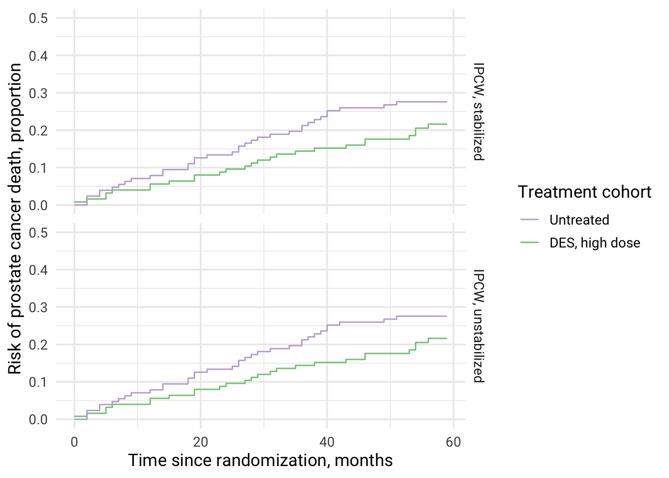
Creating IPC-weighted Aalen-Johansen survival curves for computed total effect using ggplot2
total_effect %>%
  select(`IPCW type`, cuminc_untreated, cuminc_treated) %>%
  group_by(`IPCW type`) %>%
  mutate(
    time = row_number() - 1
  ) %>%
  ungroup() %>%
  pivot_longer(
    cols = c(cuminc_untreated, cuminc_treated),
    names_to = c("cohort"),
    values_to = "cuminc_value"
  ) %>%
  ggplot(aes(x = time, y = cuminc_value, color = cohort, fill = cohort)) +
  geom_step(stat = "identity") +
  scale_y_continuous(limits = c(0,0.5)) +
  theme_minimal(base_size = 13, base_family = "Roboto") +
  scale_color_brewer(palette = "Accent", breaks=c("cuminc_untreated", "cuminc_treated"),
                     labels = c("Untreated", "DES, high dose"), guide = guide_legend(reverse = F)) +
  xlab("Time since randomization, months") +
  ylab("Risk of prostate cancer death, proportion") +
  labs(color = "Treatment cohort") +
  facet_grid(rows = vars(`IPCW type`))
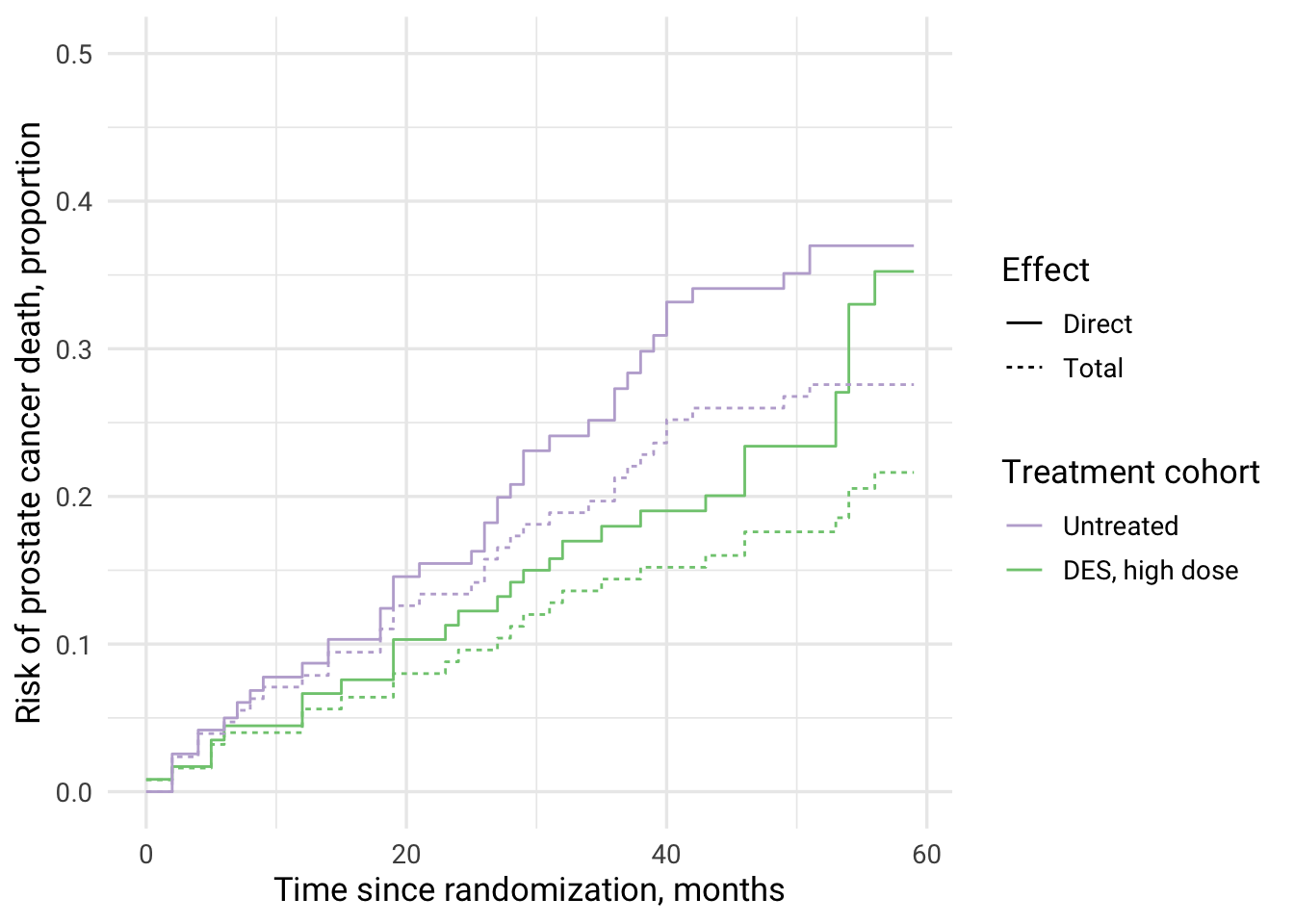
Combined figure for direct and total effects of DES on prostate cancer mortality
direct_effect %>%
  mutate(
    Effect = "Direct"
  ) %>%
  bind_rows(total_effect) %>%
  mutate(
    Effect = if_else(is.na(Effect), "Total", Effect)
  ) %>%
  select(`IPCW type`, cuminc_untreated, cuminc_treated, Effect) %>%
  filter(`IPCW type` == "IPCW, stabilized") %>%
  group_by(Effect) %>%
  mutate(
    time = row_number() - 1
  ) %>%
  ungroup() %>%
  pivot_longer(
    cols = c(cuminc_untreated, cuminc_treated),
    names_to = c("cohort"),
    values_to = "cuminc_value"
  ) %>%
  ggplot(aes(x = time, y = cuminc_value, color = cohort, fill = cohort, linetype = Effect)) +
  geom_step(stat = "identity") +
  scale_y_continuous(limits = c(0,0.5)) +
  theme_minimal(base_size = 13, base_family = "Roboto") +
  scale_color_brewer(palette = "Accent", breaks=c("cuminc_untreated", "cuminc_treated"), labels=c("Untreated", "DES, high dose"), guide = guide_legend(reverse=F)) +
  xlab("Time since randomization, months") +
  ylab("Risk of prostate cancer death, proportion") +
  labs(color = "Treatment cohort")
Computing and plotting total effect on deaths from other causes (non-prostate cancer deaths)
In this analysis, prostate cancer death is a competing event for other causes of death.
# different hazard order! now estimating effect on other causes of death and prostate cancer death becomes a competing event

#### Unstabilized
cuminc_odeath_treated_ipcw_unstab <-
  nonParametricCumInc(hazard1 = hazardO_treated_ipcw_cens_unstab,
                      hazard2 = hazard_treated_ipcw_cens_unstab,
                      competing = TRUE)

cuminc_odeath_untreated_ipcw_unstab <-
  nonParametricCumInc(hazard1 = hazardO_untreated_ipcw_cens_unstab,
                      hazard_untreated_ipcw_cens_unstab,
                      competing = TRUE)

total_effect_odeath_unstab <- bind_cols("cuminc_treated" = cuminc_odeath_treated_ipcw_unstab,
                                        "cuminc_untreated" =  cuminc_odeath_untreated_ipcw_unstab)

#### Stabilized
cuminc_odeath_treated_ipcw_stab <-
  nonParametricCumInc(hazard1 = hazardO_treated_ipcw_cens_stab,
                      hazard2 = hazard_treated_ipcw_cens_stab,
                      competing = TRUE)

cuminc_odeath_untreated_ipcw_stab <-
  nonParametricCumInc(hazard1 = hazardO_untreated_ipcw_cens_stab,
                      hazard_untreated_ipcw_cens_stab,
                      competing = TRUE)

total_effect_odeath_stab <- bind_cols("cuminc_treated" = cuminc_odeath_treated_ipcw_unstab,
                                      "cuminc_untreated" =  cuminc_odeath_untreated_ipcw_unstab)

total_effect_odeath <- list("IPCW, unstabilized" = total_effect_odeath_unstab,
                            "IPCW, stabilized" = total_effect_odeath_stab) %>%
  map(~mutate(.x,
              RR = cuminc_odeath_treated_ipcw_unstab/cuminc_odeath_untreated_ipcw_unstab,
              RD = cuminc_odeath_treated_ipcw_unstab - cuminc_odeath_untreated_ipcw_unstab
  )) %>%
  bind_rows(.id = "IPCW type")

total_effect_odeath %>%
  select(`IPCW type`, cuminc_treated, cuminc_untreated, RR, RD) %>%
  group_by(`IPCW type`) %>%
  filter(
    row_number() == 60
  ) %>%
  mutate_all(., ~round(., 2)) %>%
  ungroup() %>%
  knitr::kable()
## `mutate_all()` ignored the following grouping variables:
## • Column `IPCW type`
## ℹ Use `mutate_at(df, vars(-group_cols()), myoperation)` to silence the message.
| IPCW type | cuminc_treated | cuminc_untreated | RR | RD |
|---|---|---|---|---|
| IPCW, unstabilized | 0.51 | 0.43 | 1.19 | 0.08 |
| IPCW, stabilized | 0.51 | 0.43 | 1.19 | 0.08 |
total_effect_odeath %>%
  select(`IPCW type`, cuminc_untreated, cuminc_treated) %>%
  group_by(`IPCW type`) %>%
  mutate(
    time = row_number() - 1
  ) %>%
  ungroup() %>%
  pivot_longer(
    cols = c(cuminc_untreated, cuminc_treated),
    names_to = c("cohort"),
    values_to = "cuminc_value"
  ) %>%
  ggplot(aes(x = time, y = cuminc_value, color = cohort, fill = cohort)) +
  geom_step(stat = "identity") +
  scale_y_continuous(limits = c(0,0.5)) +
  theme_minimal(base_size = 13, base_family = "Roboto") +
  scale_color_brewer(palette = "Accent", breaks=c("cuminc_untreated", "cuminc_treated"),
                     labels = c("Untreated", "DES, high dose"), guide = guide_legend(reverse = T)) +
  xlab("Time since randomization, months") +
  ylab("Risk of other causes of death, proportion") +
  labs(color = "Treatment cohort") +
  facet_grid(rows = vars(`IPCW type`))
## Warning: Removed 6 rows containing missing values (`geom_step()`).
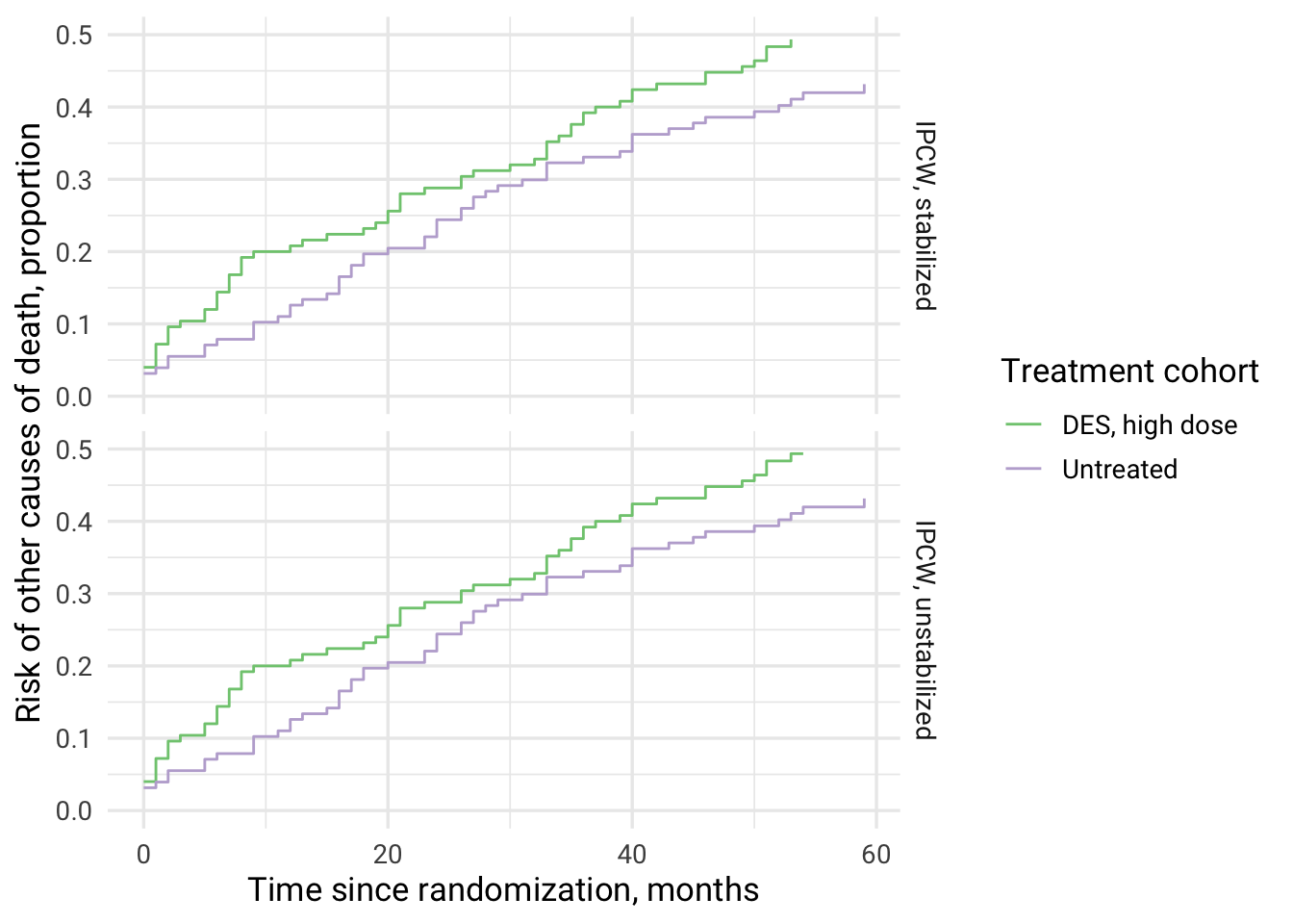
# Mortality from non-cancer causes is higher among high dose DES therapy vs no treatment (reversed from results on prostate cancer death)
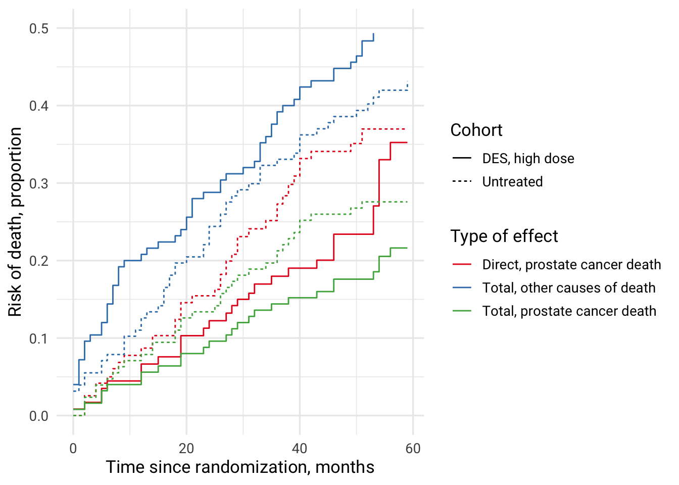
Combining all investigated effects and causes of death in one plot
direct_effect %>%
  mutate(
    Effect = "Direct, prostate cancer death"
  ) %>%
  bind_rows(total_effect) %>%
  mutate(
    Effect = if_else(is.na(Effect), "Total, prostate cancer death", Effect)
  ) %>%
  bind_rows(total_effect_odeath) %>%
  mutate(
    Effect = if_else(is.na(Effect), "Total, other causes of death", Effect)
  )  %>%
  select(`IPCW type`, cuminc_untreated, cuminc_treated, Effect) %>%
  filter(`IPCW type` == "IPCW, stabilized") %>%
  group_by(Effect) %>%
  mutate(
    time = row_number() - 1
  ) %>%
  ungroup() %>%
  pivot_longer(
    cols = c(cuminc_untreated, cuminc_treated),
    names_to = c("cohort"),
    values_to = "cuminc_value"
  ) %>%
  mutate(
    cohort = if_else(cohort == "cuminc_treated", "DES, high dose", "Untreated")
  ) %>%
  ggplot(aes(x = time, y = cuminc_value, color = Effect, fill = Effect, linetype = cohort)) +
  geom_step(stat = "identity") +
  scale_y_continuous(limits = c(0,0.5)) +
  theme_minimal(base_size = 13, base_family = "Roboto") +
  scale_color_brewer(palette = "Set1") +
  xlab("Time since randomization, months") +
  ylab("Risk of death, proportion") +
  labs(color = "Type of effect") +
  guides(linetype=guide_legend(title = "Cohort"))
## Warning: Removed 6 rows containing missing values (`geom_step()`).
Separable effects
In this part, equation (9) from Mats J. Stensrud, James M. Robins, Aaron Sarvet, Eric J. Tchetgen Tchetgen, Jessica G. Young. (2022) Conditional Separable Effects is used. Of note, identification of conditional separable effects requires additional assumptions for the causal paths of interest. Additional assumptions are introduced for the identification of the effects of interest, since (in the RCT example) only observed treatment A was factually randomized, but not the treatment components A_y and A_d, where A_y is the part of the effect of A on outcome of interest Y and A_d is the part of the effect of A on the competing events D.
This example uses cloning approach, i.e., we assign individuals to each treatment strategy at time zero.
# create variable for A_d
data_prost_long %<>% mutate(
  odeath_rx = rx
)

# Step 1: Fitting logistic regression model for the prostate cancer death
pdeath_fit <-
  glm(prostateDeath ~ rx*(dtime + I(dtime ^ 2) + I(dtime ^ 3)) + normalAct + ageCat + hx + hgBinary,
      data = data_prost_long,
      family = binomial()
    )

# Step 2: Fitting logistic regression model for other causes of death (competing event)
odeath_fit <-
  glm(otherDeath ~ odeath_rx * (dtime + I(dtime ^ 2) + I(dtime ^ 3)) + normalAct + ageCat + hx + hgBinary,
    data = data_prost_long,
    family = binomial()
    )

# Step 3: Doing cloning using long data, one data set for each level of treatment; each month of the follow-up is a row in each of the cloned data sets; baseline information has been carried forward at each time point
# each patno is repeated 60 times: T0 through end of follow-up at 60 months as saved in cutTimes vector

## Cloning for treated
data_prost_long1 <- T0 %>%
  slice(rep(1:n(), each = length(cutTimes))) %>%
  mutate(
    # create months of follow-up
    dtime = rep(cutTimes, n),
    # assign all to being treated: components of treatment are not separated
    rx = 1,
    odeath_rx = 1)

data_prost_long1 %<>% mutate(
    # predicted probability of prostate cancer death
    hazard_pdeath = predict(pdeath_fit, newdata = data_prost_long1, type = 'response'),
    # predicted probability of other death
    hazard_odeath = predict(odeath_fit, newdata = data_prost_long1, type = 'response'),
    s = (1 - hazard_pdeath) * (1 - hazard_odeath)
  )
# checks: should be 0
sum(data_prost_long1$hazard_odeath < 0)
## [1] 0
## Cloning for untreated
data_prost_long0 <- T0 %>%
  slice(rep(1:n(), each = length(cutTimes))) %>%
  mutate(
    # create months of follow-up
    dtime = rep(cutTimes, n),
    # assign all to being untreated: components of treatment are not separated
    rx = 0,
    odeath_rx = 0)

data_prost_long0 %<>% mutate(
    # predicted probability of prostate cancer death
    hazard_pdeath = predict(pdeath_fit, newdata = data_prost_long0, type = 'response'),
    # predicted probability of other death
    hazard_odeath = predict(odeath_fit, newdata = data_prost_long0, type = 'response'),
    # according to function
    s = (1 - hazard_pdeath) * (1 - hazard_odeath)
  )
# checks: should be 0
sum(data_prost_long0$hazard_odeath < 0)
## [1] 0
Perform cloning for separable causes A_y and A_d
# data set for A_Y
data_prost_long_Ay <- T0 %>%
  slice(rep(1:n(), each = length(cutTimes))) %>%
  mutate(
    # create months of follow-up
    dtime = rep(cutTimes, n),
    # assign all to being treated
    # A_y only has an effect on the prostate cancer death
    rx = 1,
    # A_d doesn't have an effect on other causes of death
    odeath_rx = 0)

data_prost_long_Ay %<>% mutate(
    # predicted probability of prostate cancer death
    hazard_pdeath = predict(pdeath_fit, newdata = data_prost_long_Ay, type = 'response'),
    # predicted probability of other death
    hazard_odeath = predict(odeath_fit, newdata = data_prost_long_Ay, type = 'response'),
    s = (1 - hazard_pdeath) * (1 - hazard_odeath)
  )
# checks: should be 0
sum(data_prost_long_Ay$hazard_odeath < 0)
## [1] 0
# Step 4: computing cumulative incidence for A=1 (A_y=1, A_d=1), A=0 (A_y=0, A_d=0), and A_y=1
cuminc_data_prost_long1 <- calculateCumInc(inputData = data_prost_long1,
                                           hazardO = "hazard_odeath",
                                           hazardP = "hazard_pdeath")
cuminc_data_prost_long0 <- calculateCumInc(inputData = data_prost_long0,
                                           hazardO = "hazard_odeath",
                                           hazardP = "hazard_pdeath")
cuminc_data_prost_long_Ay <- calculateCumInc(inputData = data_prost_long_Ay,
                                             hazardO = "hazard_odeath",
                                             hazardP = "hazard_pdeath")

cuminc_data_prost <- bind_cols("DES, high dose" = cuminc_data_prost_long1,
                               "Separable effect of DES, high dose" = cuminc_data_prost_long_Ay) %>%
  bind_cols("Untreated" = cuminc_data_prost_long0)

cuminc_data_prost %>%
  mutate(
    time = row_number() - 1
  ) %>%
  relocate(time, .before = 1) %>%
  mutate_all(~round(.x, 3)) %>%
  filter(time %in% c(12, 24, 36)) %>%
  knitr::kable()
| time | DES, high dose | Separable effect of DES, high dose | Untreated |
|---|---|---|---|
| 12 | 0.048 | 0.052 | 0.084 |
| 24 | 0.090 | 0.096 | 0.155 |
| 36 | 0.131 | 0.139 | 0.234 |
Separable effects add information on the effect of DES vs no treatment on mortality. For comparison see Table 1. Estimates of cumulative incidence after 3 years of follow-up in Conditional Separable Effects..
Create ggplot survival curves for A=1, A_y=1, and A=0 treatment regimes
cuminc_data_prost %>%
  mutate(time = row_number() - 1) %>%
  pivot_longer(cols = 1:3, names_to = "Treatment", values_to = "cuminc") %>%
  ggplot(aes(x=time, y = cuminc, color = Treatment)) +
  geom_step() +
  scale_y_continuous(limits = c(0,0.5)) +
  theme_minimal(base_size = 13, base_family = "Roboto") +
  theme(legend.position = "bottom", legend.direction = "vertical") +
  scale_color_brewer(palette = "Set2",
                     breaks = c("Untreated", "Separable effect of DES, high dose", "DES, high dose"),
                     label = c("Untreated (A_y=0, A_d=0)",
                               "Separable effect of DES, high dose (A_y=1, A_d=0)",
                               "DES, high dose (A_y=1, A_d=1)"),
                     guide = guide_legend(reverse = F)) +
  xlab("Time since randomization, months") +
  ylab("Risk of prostate cancer death, proportion")
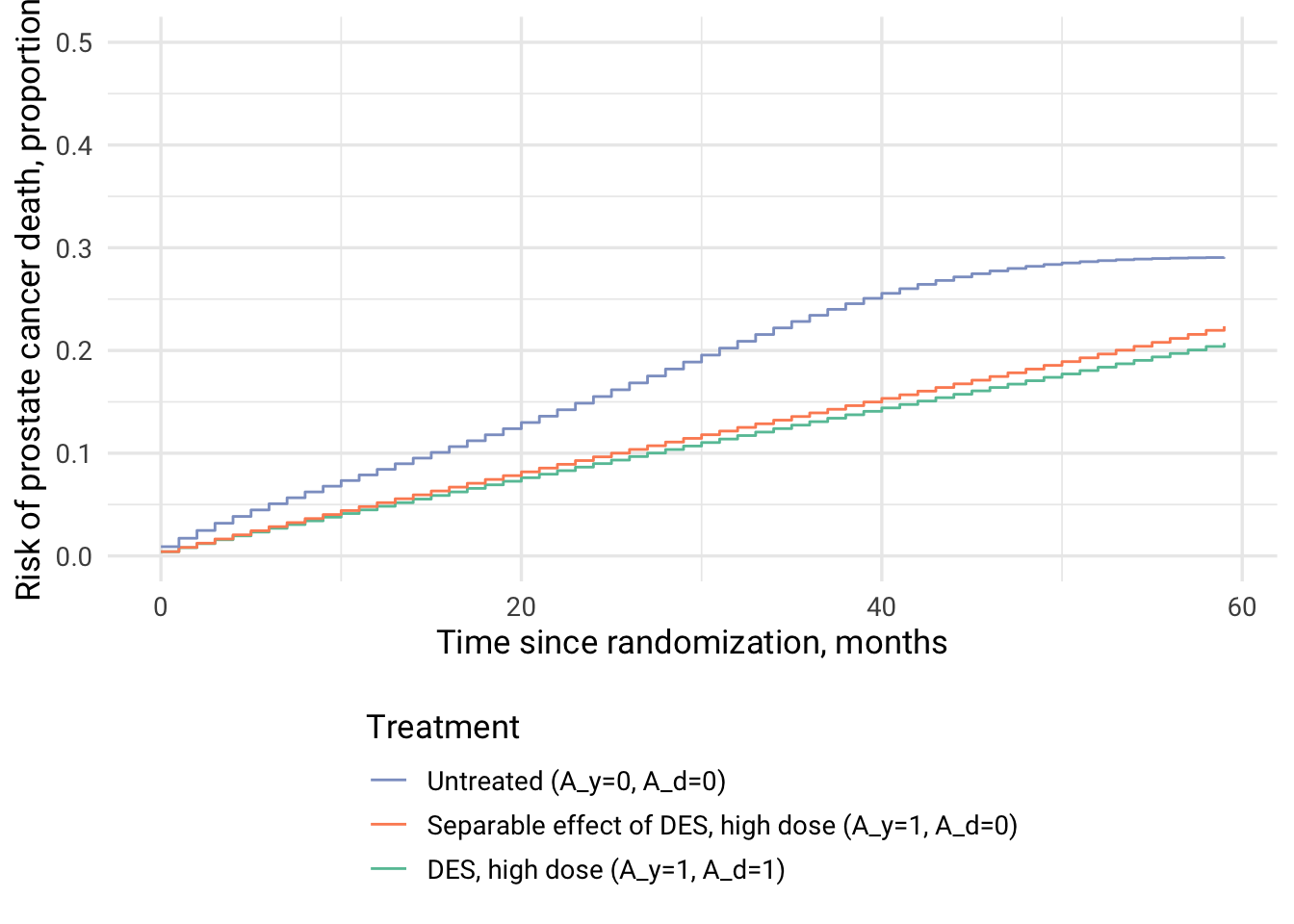
# Separable effect of DES affecting prostate cancer death
Interpretation
Previously, DES treatment vs no treatment showed reduced mortality when the direct effect on prostate cancer death was investigated, but mortality from other causes in DES cohort was increased. The interpretation of total effect of DES on prostate cancer mortality was difficult. Possible interpretation 1: prostate cancer mortality was reduced due to DES treatment and this population could die from other causes, which appeared as increased risk of death from other causes. Scenario 2: DES treatment increased mortality due to other causes and so, by being a competing event, prevented this population from dying due to prostate cancer leading to the appearance of a protective effect of DES.
The interpretation of separable effect A_y is: “the estimate of the additive indirect effect after 36 months of followup” is approx. 1% (0.138-0.129=0.009).
In my understanding, the separable effect answers the question “What is the effect of treatment on prostate cancer mortality, had the treatment, contrary to the fact, had no effect on other causes of death?”.
The causal interpretation of a separable effect A_y, like any other effect, relies on multiple assumptions, including but not limited to no unmeasured confounding between prostate cancer mortality and mortality from other causes and no unmeasured confounding for the treatment-outcome association. The latter is plausible since the example data comes from an RCT.
Take home messages
- Different effects provide different insights (i.e. answering different research questions and targeting different estimands)
- Estimation of causal direct effect requires elimination of competing events and needs to account for the loss-of-follow-up, eg, via inverse probability of censoring weighting. The estimator used to present risk curves is weighted Kaplan-Meier.
- Total effect estimation requires accounting for loss-to-follow-up but not of the competing events. The total effect includes the parts of the effect possibly mediated by the competing events (example: other than prostate cancer causes of death) and direct effect of the treatment on the prostate cancer death together. The estimator used to present risk curves is weighted Aalen-Johansen.
- Unstabilized and stabilized IPC weights performed virtually identical in this example of prostate cancer death data from Byar & Greene’s DES treatment RCT.
- Separable effects of time-fixed exposure (point exposure) on the outcome can provide additional information on the effects of interest. Separable effect of an exposure refers to “decomposition” of a treatment into “distinct components”, where each exposure component can be assigned distinct and different values.
References
- Base R code by Paloma Rojas-Saunero, PhD
here, which served as a basis for the
tidyversecode here. - Stensrud, M.J., Hernán, M.A., Tchetgen Tchetgen, E.J. et al. A generalized theory of separable effects in competing event settings. Lifetime Data Anal 27, 588–631 (2021). https://doi.org/10.1007/s10985-021-09530-8
- Mats J. Stensrud, Oliver Dukes. (2022) Translating questions to estimands in randomized clinical trials with intercurrent events. Statistics in Medicine 41:16, pages 3211-3228.
- Young, JG, Stensrud, MJ, Tchetgen Tchetgen, EJ, Hernán, MA. A causal framework for classical statistical estimands in failure-time settings with competing events. Statistics in Medicine. 2020; 39: 1199– 1236. https://doi.org/10.1002/sim.8471
- Mats J. Stensrud, James M. Robins, Aaron Sarvet, Eric J. Tchetgen Tchetgen, Jessica G. Young. (2022) Conditional Separable Effects. Journal of the American Statistical Association 0:0, pages 1-13.
- Young JG, Stensrud MJ. Identified Versus Interesting Causal Effects in Fertility Trials and Other Settings With Competing or Truncation Events. Epidemiology. 2021 Jul 1;32(4):569-572. doi: 10.1097/EDE.0000000000001357. PMID: 34042075.
- Rojas-Saunero LP, Young JG, Didelez V, Ikram MA, Swanson SA. Choosing questions before methods in dementia research with competing events and causal goals. Published online June 3, 2021:2021.06.01.21258142. doi:10.1101/2021.06.01.21258142