Using `WeightIt` R package for causal inference analyses
I recently discovered WeightIt
R package and was very happy with its functionality and performance. I “delegated” my code computing IPTW to WeightIt and it was faster while producing the same results, as expected. In this post I will use publicly available data to demonstrate the great functionality of WeightIt and the scope of challenges it may help addressing.
Open data
temp <- tempfile()

temp2 <- tempfile()

download.file("https://cdn1.sph.harvard.edu/wp-content/uploads/sites/1268/2017/01/nhefs_excel.zip", temp)

unzip(zipfile = temp, exdir = temp2)

data <- readxl::read_xls(file.path(temp2, "NHEFS.xls"))

unlink(c(temp, temp2))

data
## # A tibble: 1,629 × 64
##     seqn  qsmk death yrdth modth dadth   sbp   dbp   sex   age  race income
##    <dbl> <dbl> <dbl> <dbl> <dbl> <dbl> <dbl> <dbl> <dbl> <dbl> <dbl>  <dbl>
##  1   233     0     0    NA    NA    NA   175    96     0    42     1     19
##  2   235     0     0    NA    NA    NA   123    80     0    36     0     18
##  3   244     0     0    NA    NA    NA   115    75     1    56     1     15
##  4   245     0     1    85     2    14   148    78     0    68     1     15
##  5   252     0     0    NA    NA    NA   118    77     0    40     0     18
##  6   257     0     0    NA    NA    NA   141    83     1    43     1     11
##  7   262     0     0    NA    NA    NA   132    69     1    56     0     19
##  8   266     0     0    NA    NA    NA   100    53     1    29     0     22
##  9   419     0     1    84    10    13   163    79     0    51     0     18
## 10   420     0     1    86    10    17   184   106     0    43     0     16
## # … with 1,619 more rows, and 52 more variables: marital <dbl>, school <dbl>,
## #   education <dbl>, ht <dbl>, wt71 <dbl>, wt82 <dbl>, wt82_71 <dbl>,
## #   birthplace <dbl>, smokeintensity <dbl>, smkintensity82_71 <dbl>,
## #   smokeyrs <dbl>, asthma <dbl>, bronch <dbl>, tb <dbl>, hf <dbl>, hbp <dbl>,
## #   pepticulcer <dbl>, colitis <dbl>, hepatitis <dbl>, chroniccough <dbl>,
## #   hayfever <dbl>, diabetes <dbl>, polio <dbl>, tumor <dbl>,
## #   nervousbreak <dbl>, alcoholpy <dbl>, alcoholfreq <dbl>, …
For this section, I will partly re-use the code by Joy Shi and Sean McGrath available here.
data %<>%
  mutate(
    # define censoring
    cens = if_else(is.na(wt82_71),1, 0),
    # categorize the school variable (as in R code by Joy Shi and Sean McGrath)
    education = cut(school, breaks = c(0, 8, 11, 12, 15, 20),
                    include.lowest = TRUE,
                    labels = c('1. 8th Grage or Less',
                               '2. HS Dropout',
                               '3. HS',
                               '4. College Dropout',
                               '5. College or More')),
    # establish active as a factor variable
    active = factor(active),
    # establish exercise as a factor variable
    exercise = factor(exercise),
    # create a treatment label variable
    qsmklabel = if_else(qsmk == 1,
                        'Quit Smoking 1971-1982',
                        'Did Not Quit Smoking 1971-1982'),
  # survtime variable
  survtime = if_else(death == 0, 120, (yrdth-83)*12 + modth) # yrdth ranges from 83 to 92
    ) %>%
  # ignore those with missing values on some variables
  filter(!is.na(education))
Descriptive table with balancing characteristics
table <- bal.tab(death ~ qsmk + sex + race + age + education + smokeintensity + smkintensity82_71 + smokeyrs + exercise + active + wt71, data = data, estimand = "ATE", thresholds = c(m = 0.1))

table
## Balance Measures
##                                   Type Diff.Un     M.Threshold.Un
## qsmk                            Binary  0.0721     Balanced, <0.1
## sex                             Binary -0.1525 Not Balanced, >0.1
## race                            Binary  0.0275     Balanced, <0.1
## age                            Contin.  1.3419 Not Balanced, >0.1
## education_1. 8th Grage or Less  Binary  0.2356 Not Balanced, >0.1
## education_2. HS Dropout         Binary  0.0136     Balanced, <0.1
## education_3. HS                 Binary -0.1705 Not Balanced, >0.1
## education_4. College Dropout    Binary -0.0297     Balanced, <0.1
## education_5. College or More    Binary -0.0490     Balanced, <0.1
## smokeintensity                 Contin.  0.0195     Balanced, <0.1
## smkintensity82_71              Contin. -0.2598 Not Balanced, >0.1
## smokeyrs                       Contin.  1.2315 Not Balanced, >0.1
## exercise_0                      Binary -0.0464     Balanced, <0.1
## exercise_1                      Binary -0.0788     Balanced, <0.1
## exercise_2                      Binary  0.1252 Not Balanced, >0.1
## active_0                        Binary -0.0950     Balanced, <0.1
## active_1                        Binary  0.0466     Balanced, <0.1
## active_2                        Binary  0.0484     Balanced, <0.1
## wt71                           Contin.  0.1181 Not Balanced, >0.1
##
## Balance tally for mean differences
##                    count
## Balanced, <0.1        11
## Not Balanced, >0.1     8
##
## Variable with the greatest mean difference
##  Variable Diff.Un     M.Threshold.Un
##       age  1.3419 Not Balanced, >0.1
##
## Sample sizes
##     Control Treated
## All    1311     318
Several important covariables are unbalanced with standardized mean difference > 10% (SMD > 0.1), e.g., sex, age, education, previous weight wt71, previous smoking intensity and duration, and psychical activity level. Not adressing confounding by these factors, we cannot estimate the true average causal effect (ATE) of smoking cessation qsmk on mortality
Computing inverse probability of treatment weights for the point treatment
iptw <- weightit(qsmk ~ sex + race + age + I(age*age) + as.factor(education) + smokeintensity + I(smokeintensity*smokeintensity) + smokeyrs + I(smokeyrs*smokeyrs) + as.factor(exercise) + as.factor(active) + wt71 + I(wt71*wt71), data = data, estimand = "ATE", method = "ps")

iptw
## A weightit object
##  - method: "ps" (propensity score weighting)
##  - number of obs.: 1629
##  - sampling weights: none
##  - treatment: 2-category
##  - estimand: ATE
##  - covariates: sex, race, age, I(age * age), as.factor(education), smokeintensity, I(smokeintensity * smokeintensity), smokeyrs, I(smokeyrs * smokeyrs), as.factor(exercise), as.factor(active), wt71, I(wt71 * wt71)
summary(iptw)
##                  Summary of weights
##
## - Weight ranges:
##
##            Min                                   Max
## treated 1.2607 |---------------------------| 16.0062
## control 1.0559 |--|                           2.9229
##
## - Units with 5 most extreme weights by group:
##
##             1551    1503    1244   1376     170
##  treated 10.1178 11.0187 12.3286  15.82 16.0062
##              722     633     774   1229    1088
##  control  2.5007  2.5423  2.6693 2.8155  2.9229
##
## - Weight statistics:
##
##         Coef of Var   MAD Entropy # Zeros
## treated       0.475 0.334   0.095       0
## control       0.171 0.122   0.013       0
##
## - Effective Sample Sizes:
##
##            Control Treated
## Unweighted 1201.    428.
## Weighted   1166.82  349.46
There are no extreme weights; the exposed vs unexposed counts in the raw and weighted populations are presented. Now we can investigate how much we improved the exchangeability between exposed and unexposed by re-weighting the original population using computed IPTW.
table_iptw <- bal.tab(iptw, stats = c("m"), thresholds = c(m = 0.01))

table_iptw
## Call
##  weightit(formula = qsmk ~ sex + race + age + I(age * age) + as.factor(education) +
##     smokeintensity + I(smokeintensity * smokeintensity) + smokeyrs +
##     I(smokeyrs * smokeyrs) + as.factor(exercise) + as.factor(active) +
##     wt71 + I(wt71 * wt71), data = data, method = "ps", estimand = "ATE")
##
## Balance Measures
##                                               Type Diff.Adj         M.Threshold
## prop.score                                Distance   0.0081     Balanced, <0.01
## sex                                         Binary  -0.0010     Balanced, <0.01
## race                                        Binary   0.0025     Balanced, <0.01
## age                                        Contin.   0.0022     Balanced, <0.01
## I(age * age)                               Contin.   0.0023     Balanced, <0.01
## as.factor(education)_1. 8th Grage or Less   Binary  -0.0093     Balanced, <0.01
## as.factor(education)_2. HS Dropout          Binary   0.0013     Balanced, <0.01
## as.factor(education)_3. HS                  Binary   0.0011     Balanced, <0.01
## as.factor(education)_4. College Dropout     Binary   0.0059     Balanced, <0.01
## as.factor(education)_5. College or More     Binary   0.0009     Balanced, <0.01
## smokeintensity                             Contin.  -0.0226 Not Balanced, >0.01
## I(smokeintensity * smokeintensity)         Contin.  -0.0254 Not Balanced, >0.01
## smokeyrs                                   Contin.  -0.0040     Balanced, <0.01
## I(smokeyrs * smokeyrs)                     Contin.  -0.0013     Balanced, <0.01
## as.factor(exercise)_0                       Binary  -0.0038     Balanced, <0.01
## as.factor(exercise)_1                       Binary   0.0188 Not Balanced, >0.01
## as.factor(exercise)_2                       Binary  -0.0149 Not Balanced, >0.01
## as.factor(active)_0                         Binary  -0.0064     Balanced, <0.01
## as.factor(active)_1                         Binary   0.0122 Not Balanced, >0.01
## as.factor(active)_2                         Binary  -0.0058     Balanced, <0.01
## wt71                                       Contin.   0.0019     Balanced, <0.01
## I(wt71 * wt71)                             Contin.   0.0047     Balanced, <0.01
##
## Balance tally for mean differences
##                     count
## Balanced, <0.01        17
## Not Balanced, >0.01     5
##
## Variable with the greatest mean difference
##                            Variable Diff.Adj         M.Threshold
##  I(smokeintensity * smokeintensity)  -0.0254 Not Balanced, >0.01
##
## Effective sample sizes
##            Control Treated
## Unadjusted 1201.    428.
## Adjusted   1166.82  349.46
An important covariable smokeintensity remained unbalanced; however, there is a clear exchangeability improvement (less confounding) in the re-weighted population vs original one (wrt sex, age, physical activity variables and previous weight wt71).
We can run a weighted Cox proportional hazards regression model using computed weights.
# crude Cox PH model
cox_model_crude <- coxph(Surv(survtime, death == 1) ~ qsmk, data = data)
cox_fit_crude  <- cox_model_crude %>% broom::tidy(., conf.int = T, exponentiate = T)

# IPTW Cox PH model
cox_model_iptw <- coxph(Surv(survtime, death == 1) ~ qsmk, data = data, weights = iptw$weights)
cox_fit_iptw  <- cox_model_iptw %>% broom::tidy(., conf.int = T, exponentiate = T)

# HR
cox_fit_crude %>% bind_rows(cox_fit_iptw)
## # A tibble: 2 × 8
##   term  estimate std.error statistic p.value conf.low conf.high robust.se
##   <chr>    <dbl>     <dbl>     <dbl>   <dbl>    <dbl>     <dbl>     <dbl>
## 1 qsmk      1.39    0.120    2.77    0.00565    1.10       1.76    NA
## 2 qsmk      1.00    0.0795   0.00883 0.993      0.770      1.30     0.134
Next, I compute 95% CIs using bootsrap percentiles.
library(tidymodels)
## Registered S3 method overwritten by 'tune':
##   method                   from
##   required_pkgs.model_spec parsnip
## ── Attaching packages ────────────────────────────────────── tidymodels 0.1.4 ──
## ✓ broom        0.7.10     ✓ rsample      0.1.1
## ✓ dials        0.0.10     ✓ tune         0.1.6
## ✓ infer        1.0.0      ✓ workflows    0.2.4
## ✓ modeldata    0.1.1      ✓ workflowsets 0.1.0
## ✓ parsnip      0.1.7      ✓ yardstick    0.0.9
## ✓ recipes      0.1.17
## ── Conflicts ───────────────────────────────────────── tidymodels_conflicts() ──
## x scales::discard()       masks purrr::discard()
## x magrittr::extract()     masks tidyr::extract()
## x dplyr::filter()         masks stats::filter()
## x recipes::fixed()        masks stringr::fixed()
## x dplyr::lag()            masks stats::lag()
## x rsample::permutations() masks gtools::permutations()
## x MASS::select()          masks dplyr::select()
## x magrittr::set_names()   masks purrr::set_names()
## x yardstick::spec()       masks readr::spec()
## x recipes::step()         masks stats::step()
## • Use tidymodels_prefer() to resolve common conflicts.
times <- 1e3 # 1K samples
set.seed(876434567)
boots <- bootstraps(data, times = times, apparent = FALSE)

# function to plug-in the sampled data sets
cox_model <- function(data, iptw) {
  coxph(Surv(survtime, death == 1) ~ qsmk, data = data, weights = iptw$weights)
}

boot_models <- boots %>%
  mutate(
    # explicitly transform sampled datasets/splits to tibbles
    splits = map(splits, ~as_tibble(.x)),
    # compute IPTW in each split/sampled data set
    iptw = map(splits, ~weightit(qsmk ~ sex + race + age + I(age*age) + as.factor(education) + smokeintensity + I(smokeintensity*smokeintensity) + smokeyrs + I(smokeyrs*smokeyrs) + as.factor(exercise) + as.factor(active) + wt71 + I(wt71*wt71), data = .x, estimand = "ATE", method = "ps")),
    # using each data sample and corresponding IPTWs, run weighted Cox PH model
    model = map2(.x = splits, .y = iptw, ~cox_model(data = .x, iptw = .y)),
    coef_info = map(model, ~broom::tidy(.x, exponentiate = T)))

# combine coefficients from all sampled data sets in one tibble
boot_coefs <- boot_models %>%
  unnest(coef_info)

# compute 95% CI using all sampled data sets results
percentile_intervals <- boot_coefs %>%
  summarise_at(.vars = vars(estimate),
               .funs = list(Q2.5 = ~ quantile(., probs = 0.025), # lower bound of 95% CI
                            Q50 = ~ quantile(., probs = 0.50), # point estimate
                            Q97.5 = ~ quantile(., probs = 0.975))) # upper bound of 95% CI

percentile_intervals
## # A tibble: 1 × 3
##    Q2.5   Q50 Q97.5
##   <dbl> <dbl> <dbl>
## 1 0.802 0.998  1.24
Overall, we found no effect of smoking cessation on mortality at the end of data at t=120 months.
Simulated data
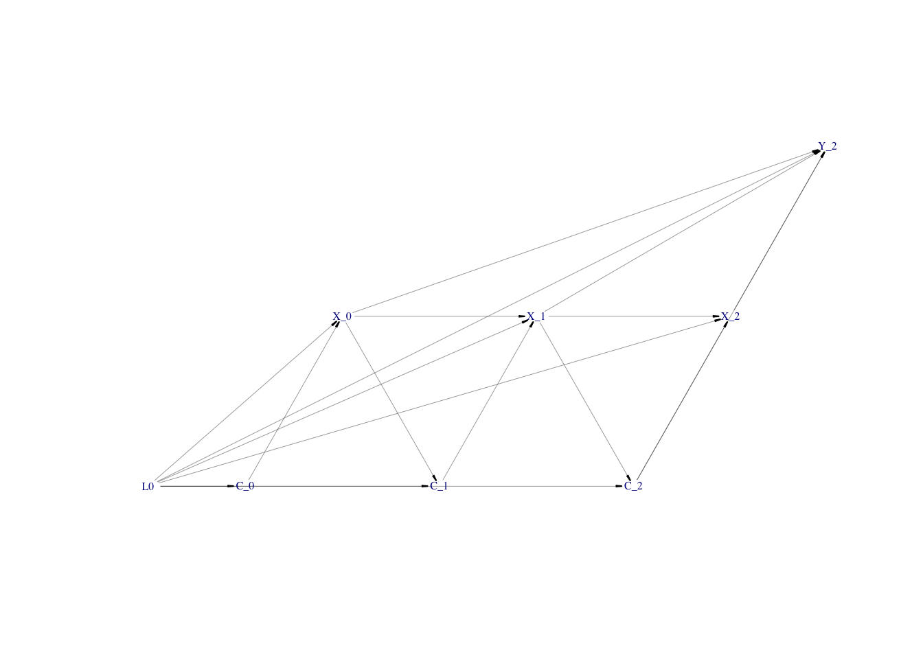
First, I will use the example of the simulated time-varying confounding and exposure using simcausal
package vignette. I reduce the number of time points to 3 (see the final directed acyclic graph presenting the simulated data), simulate one cumulative outcome at the end of data at t=2 and add effects of previous exposures X on the cumulative outcome at t=2 (see DAG).
library(simcausal)

D <- DAG.empty() +
  node("L0", distr = "rcat.b1", probs = c(0.5, 0.25, 0.25)) +
  node("C", t = 0, distr = "rnorm", mean = 3 + (L0 > 1) * 3 + (L0 > 2) * 3) +
  node("X", t = 0, distr = "rbern", prob = plogis(0.2 + 0.3 * L0 + 0.5 * C[t])) +

  node("C", t = 1:2, distr = "rnorm", mean = -X[t-1]*10 + 5 + (L0 > 1) * 3 + (L0 > 2) * 2) +
  node("X", t = 1:2, distr = "rbern", prob = plogis(0.1 + 0.1 * L0 + 0.4 * C[t] + 2 * X[t - 1])) +
  node("Y", t = 2, distr = "rbern", prob = plogis(0.1 + 1.2 * X[t] + 1.3 * X[t-1] + 1.1 * X[t-2] + 0.1 * L0 + 0.2 * C[t]), EFU = TRUE)

D <- set.DAG(D)
## ...automatically assigning order attribute to some nodes...
## node L0, order:1
## node C_0, order:2
## node X_0, order:3
## node C_1, order:4
## node X_1, order:5
## node C_2, order:6
## node X_2, order:7
## node Y_2, order:8
plotDAG(D)
## using the following vertex attributes:
## NAdarkbluenone70.50
## using the following edge attributes:
## black0.210.30.2
dat.long <- sim(D, n = 3e3)
## simulating observed dataset from the DAG object
# NAs are not allowed for exposure nodes; I want to code L0 explicitly as a factor with 3 levels and not as continuous variable
dat.long %<>%
  filter(!is.na(X_0)) %>%
  filter(!is.na(X_1)) %>%
  filter(!is.na(X_2)) %>%
  mutate(
    L0 = as.factor(L0)
  )
Using WeightIt, I will compute the total effect of exposure X at t=0, t=1 and t=2 on the outcome Y while adjusting for the time-varying confounder C. But first, I check the covariables balance at every time-point in the time-varying simulated data set.
balance_tab <- bal.tab(list(X_0 ~ L0 + C_0,
             X_1 ~ X_0 + L0 + C_1,
             X_2 ~ X_0 + X_1 + L0 + C_1 + C_2),
        data = dat.long, stats = c("m"), thresholds = c(m = 0.1),
        which.time = .all)

balance_tab
## Balance by Time Point
##
##  - - - Time: 1 - - -
## Balance Measures
##         Type Diff.Un     M.Threshold.Un
## L0_1  Binary -0.4477 Not Balanced, >0.1
## L0_2  Binary  0.1983 Not Balanced, >0.1
## L0_3  Binary  0.2494 Not Balanced, >0.1
## C_0  Contin.  1.1548 Not Balanced, >0.1
##
## Balance tally for mean differences
##                    count
## Balanced, <0.1         0
## Not Balanced, >0.1     4
##
## Variable with the greatest mean difference
##  Variable Diff.Un     M.Threshold.Un
##       C_0  1.1548 Not Balanced, >0.1
##
## Sample sizes
##     Control Treated
## All     222    2778
##
##  - - - Time: 2 - - -
## Balance Measures
##         Type Diff.Un     M.Threshold.Un
## X_0   Binary -0.0654     Balanced, <0.1
## L0_1  Binary -0.3346 Not Balanced, >0.1
## L0_2  Binary  0.0939     Balanced, <0.1
## L0_3  Binary  0.2408 Not Balanced, >0.1
## C_1  Contin.  0.9073 Not Balanced, >0.1
##
## Balance tally for mean differences
##                    count
## Balanced, <0.1         2
## Not Balanced, >0.1     3
##
## Variable with the greatest mean difference
##  Variable Diff.Un     M.Threshold.Un
##       C_1  0.9073 Not Balanced, >0.1
##
## Sample sizes
##     Control Treated
## All     826    2174
##
##  - - - Time: 3 - - -
## Balance Measures
##         Type Diff.Un     M.Threshold.Un
## X_0   Binary  0.0722     Balanced, <0.1
## X_1   Binary -0.2291 Not Balanced, >0.1
## L0_1  Binary -0.2453 Not Balanced, >0.1
## L0_2  Binary  0.0482     Balanced, <0.1
## L0_3  Binary  0.1971 Not Balanced, >0.1
## C_1  Contin.  0.0915     Balanced, <0.1
## C_2  Contin.  0.9404 Not Balanced, >0.1
##
## Balance tally for mean differences
##                    count
## Balanced, <0.1         3
## Not Balanced, >0.1     4
##
## Variable with the greatest mean difference
##  Variable Diff.Un     M.Threshold.Un
##       C_2  0.9404 Not Balanced, >0.1
##
## Sample sizes
##     Control Treated
## All     634    2366
##  - - - - - - - - - - -
Evidently, the farther observations are from the baseline t=0, the more imbalance there is.
Next, I will construct PS models for every time point in the data set to compute IPTWs.
iptw_models <- weightitMSM(list(X_0 ~ L0 + C_0,
                                X_1 ~ X_0 + L0 + C_1,
                                X_2 ~ X_0 + X_1 + L0 + C_1 + C_2),
                           data = dat.long, method = "ps", stabilize = TRUE)
iptw_models
## A weightitMSM object
##  - method: "ps" (propensity score weighting)
##  - number of obs.: 3000
##  - sampling weights: none
##  - number of time points: 3 (X_0, X_1, X_2)
##  - treatment:
##     + time 1: 2-category
##     + time 2: 2-category
##     + time 3: 2-category
##  - covariates:
##     + baseline: L0, C_0
##     + after time 1: X_0, L0, C_1
##     + after time 2: X_0, X_1, L0, C_1, C_2
##  - stabilized; stabilization factors:
##     + baseline: (none)
##     + after time 1: X_0
##     + after time 2: X_0, X_1, X_0:X_1
summary(iptw_models)
##                  Summary of weights
##
##                        Time 1
##                  Summary of weights
##
## - Weight ranges:
##
##            Min                                   Max
## treated 0.2488  |--------------------|        9.0953
## control 0.1173 |---------------------------| 11.3726
##
## - Units with 5 most extreme weights by group:
##
##            1492    389   1916    392     426
##  treated 5.1977 5.4518 5.4809 6.0153  9.0953
##            1140     71    130    149     950
##  control 6.5338 6.9171  8.839 9.6473 11.3726
##
## - Weight statistics:
##
##         Coef of Var   MAD Entropy # Zeros
## treated       0.650 0.450   0.158       0
## control       1.605 0.773   0.600       0
##
## - Mean of Weights = 0.99
##
## - Effective Sample Sizes:
##
##            Control Treated
## Unweighted  222.   2778.
## Weighted     62.27 1953.57
##
##                        Time 2
##                  Summary of weights
##
## - Weight ranges:
##
##            Min                                   Max
## treated 0.1173 |---------------------------| 11.3726
## control 0.1215 |---------------------|        9.0953
##
## - Units with 5 most extreme weights by group:
##
##            1140     71    130    149     950
##  treated 6.5338 6.9171  8.839 9.6473 11.3726
##            1492    389   1916    392     426
##  control 5.1977 5.4518 5.4809 6.0153  9.0953
##
## - Weight statistics:
##
##         Coef of Var   MAD Entropy # Zeros
## treated       0.711 0.462   0.173       0
## control       0.833 0.503   0.227       0
##
## - Mean of Weights = 0.99
##
## - Effective Sample Sizes:
##
##            Control Treated
## Unweighted   826.  2174.
## Weighted     487.9 1443.92
##
##                        Time 3
##                  Summary of weights
##
## - Weight ranges:
##
##            Min                                   Max
## treated 0.1215 |-----------------------|      9.6473
## control 0.1173 |---------------------------| 11.3726
##
## - Units with 5 most extreme weights by group:
##
##            1140     71   130    426     149
##  treated 6.5338 6.9171 8.839 9.0953  9.6473
##            2363   1666    65   1688     950
##  control 3.5002 3.5116 3.523 5.2801 11.3726
##
## - Weight statistics:
##
##         Coef of Var   MAD Entropy # Zeros
## treated       0.749 0.493   0.193       0
## control       0.728 0.397   0.166       0
##
## - Mean of Weights = 0.99
##
## - Effective Sample Sizes:
##
##            Control Treated
## Unweighted  634.   2366.
## Weighted    414.75 1515.35
No extreme weights were produced. Now I will check the covariables balance when the population is reweighted at each time point by the IPT weights computed above.
balance_tab_iptw <- bal.tab(iptw_models, stats = c("m"), thresholds = c(m = 0.1),
        which.time = .all)

balance_tab_iptw
## Call
##  weightitMSM(formula.list = list(X_0 ~ L0 + C_0, X_1 ~ X_0 + L0 +
##     C_1, X_2 ~ X_0 + X_1 + L0 + C_1 + C_2), data = dat.long,
##     method = "ps", stabilize = TRUE)
##
## Balance by Time Point
##
##  - - - Time: 1 - - -
## Balance Measures
##                Type Diff.Adj        M.Threshold
## prop.score Distance   0.0837     Balanced, <0.1
## L0_1         Binary  -0.0443     Balanced, <0.1
## L0_2         Binary  -0.0261     Balanced, <0.1
## L0_3         Binary   0.0705     Balanced, <0.1
## C_0         Contin.   0.1405 Not Balanced, >0.1
##
## Balance tally for mean differences
##                    count
## Balanced, <0.1         4
## Not Balanced, >0.1     1
##
## Variable with the greatest mean difference
##  Variable Diff.Adj        M.Threshold
##       C_0   0.1405 Not Balanced, >0.1
##
## Effective sample sizes
##            Control Treated
## Unadjusted  222.   2778.
## Adjusted     62.27 1953.57
##
##  - - - Time: 2 - - -
## Balance Measures
##                Type Diff.Adj        M.Threshold
## prop.score Distance   0.1068
## X_0          Binary  -0.0707     Balanced, <0.1
## L0_1         Binary  -0.0049     Balanced, <0.1
## L0_2         Binary   0.0043     Balanced, <0.1
## L0_3         Binary   0.0006     Balanced, <0.1
## C_1         Contin.   0.2591 Not Balanced, >0.1
##
## Balance tally for mean differences
##                    count
## Balanced, <0.1         4
## Not Balanced, >0.1     1
##
## Variable with the greatest mean difference
##  Variable Diff.Adj        M.Threshold
##       C_1   0.2591 Not Balanced, >0.1
##
## Effective sample sizes
##            Control Treated
## Unadjusted   826.  2174.
## Adjusted     487.9 1443.92
##
##  - - - Time: 3 - - -
## Balance Measures
##                Type Diff.Adj        M.Threshold
## prop.score Distance   0.4357
## X_0          Binary   0.0452     Balanced, <0.1
## X_1          Binary  -0.2512 Not Balanced, >0.1
## L0_1         Binary  -0.0258     Balanced, <0.1
## L0_2         Binary  -0.0169     Balanced, <0.1
## L0_3         Binary   0.0426     Balanced, <0.1
## C_1         Contin.  -0.0709     Balanced, <0.1
## C_2         Contin.   0.6987 Not Balanced, >0.1
##
## Balance tally for mean differences
##                    count
## Balanced, <0.1         5
## Not Balanced, >0.1     2
##
## Variable with the greatest mean difference
##  Variable Diff.Adj        M.Threshold
##       C_2   0.6987 Not Balanced, >0.1
##
## Effective sample sizes
##            Control Treated
## Unadjusted  634.   2366.
## Adjusted    414.75 1515.35
##  - - - - - - - - - - -
Although IPT weighting meaningfully improved covariables' balance, for confounder C at t=1, SMD indicated distribution imbalance for confounder C at t=2 and several other variables, which serves as the evidence of corrupted conditional exchangeability (residual confounding is present).
library(survey)
## Loading required package: grid
## Loading required package: Matrix
##
## Attaching package: 'Matrix'
## The following objects are masked from 'package:tidyr':
##
##     expand, pack, unpack
##
## Attaching package: 'survey'
## The following object is masked from 'package:graphics':
##
##     dotchart
res_svy <- svydesign(~1, weights = iptw_models$weights, data = dat.long)

res_svy_full <- svyglm(Y_2 ~ X_0 * X_1 * X_2, design = res_svy)
res_svy_full %>% broom::tidy(exponentiate = T, conf.int = T)
## # A tibble: 8 × 7
##   term        estimate std.error statistic  p.value conf.low conf.high
##   <chr>          <dbl>     <dbl>     <dbl>    <dbl>    <dbl>     <dbl>
## 1 (Intercept)    2.72   2.36e-13  4.24e+12 0           2.72      2.72
## 2 X_0            0.972  2.10e- 2 -1.38e+ 0 0.169       0.932     1.01
## 3 X_1            0.841  5.13e- 2 -3.37e+ 0 0.000749    0.761     0.930
## 4 X_2            0.954  3.69e- 2 -1.27e+ 0 0.204       0.888     1.03
## 5 X_0:X_1        1.06   5.79e- 2  1.01e+ 0 0.313       0.946     1.19
## 6 X_0:X_2        1.05   4.29e- 2  1.11e+ 0 0.266       0.964     1.14
## 7 X_1:X_2        1.14   6.94e- 2  1.82e+ 0 0.0681      0.991     1.30
## 8 X_0:X_1:X_2    0.985  7.49e- 2 -1.97e- 1 0.844       0.851     1.14
main_effects <- svyglm(Y_2 ~ X_0 + X_1 + X_2, design = res_svy)
main_effects  %>% broom::tidy(exponentiate = T, conf.int = T)
## # A tibble: 4 × 7
##   term        estimate std.error statistic   p.value conf.low conf.high
##   <chr>          <dbl>     <dbl>     <dbl>     <dbl>    <dbl>     <dbl>
## 1 (Intercept)    2.29    0.0286      28.9  1.96e-162    2.16       2.42
## 2 X_0            1.05    0.0248       2.04 4.16e-  2    1.00       1.10
## 3 X_1            0.988   0.00807     -1.48 1.40e-  1    0.973      1.00
## 4 X_2            1.11    0.0156       6.39 1.88e- 10    1.07       1.14
cum_fit <- svyglm(Y_2 ~ I(X_0 + X_1 + X_2), design = res_svy)
cum_fit %>% broom::tidy(exponentiate = T, conf.int = T)
## # A tibble: 2 × 7
##   term               estimate std.error statistic   p.value conf.low conf.high
##   <chr>                 <dbl>     <dbl>     <dbl>     <dbl>    <dbl>     <dbl>
## 1 (Intercept)            2.32   0.0216      39.0  2.16e-269     2.22      2.42
## 2 I(X_0 + X_1 + X_2)     1.04   0.00816      5.19 2.21e-  7     1.03      1.06
On the relative scale, the cumulative effect of 3 doses of exposure X was associated with 4% increased risk of Y at the time t=2 (end of data). Had this analysis been based on non-simulated data, the detailed interpretation of this measure of effect would depend on the research question and domain expertise. Since this was an example using simulated data set with no true underlying clinical or otherwise practical and socially important research question, I get to claim that 4% increased risk does not warranty any concern.
Take home message
WeightIt
R package is great. It increased my quality of research life by sparing me the additional “by hand” coding. I am sure it is and will be useful for many research folks out there ✌️
Cheers! ✌️
References
- Hernán MA, Robins JM (2020). Causal Inference: What If. Boca Raton: Chapman & Hall/CRC
- R code by Joy Shi and Sean McGrath available here
WeightItR package: https://cran.r-project.org/web/packages/WeightIt/index.htmlsimcausalR package: https://github.com/osofr/simcausal- Austin, Peter C. 2011. “An Introduction to Propensity Score Methods for Reducing the Effects of Confounding in Observational Studies.” Multivariate Behavioral Research 46 (3): 399–424. https://doi.org/10.1080/00273171.2011.568786.
- Austin, Peter C., and Elizabeth A. Stuart. 2015. “Moving Towards Best Practice When Using Inverse Probability of Treatment Weighting (IPTW) Using the Propensity Score to Estimate Causal Treatment Effects in Observational Studies.” Statistics in Medicine 34 (28): 3661–79. https://doi.org/10.1002/sim.6607