Bootstrapping and plotting 95% confidence bands: 'Causal Inference: What If' Causal Survival Analysis. Parametric g-formula

In this post, I explore parametric g-formula fitting in the causal survival analysis context. I use the machinery of the tidyverse throughout the post and finish with plotting the 95% confidence band around the g-formula fitted survival curve for smokers vs non-smokers (see Chapter 17, Hernán MA, Robins JM (2020). Causal Inference: What If. Boca Raton: Chapman & Hall/CRC).

Getting the data

library(tidyverse)
library(magrittr)
library(conflicted)  
library(readxl)
library(wesanderson)
library(patchwork)

conflict_prefer("filter", "dplyr")

temp <- tempfile()

temp2 <- tempfile()

download.file("https://cdn1.sph.harvard.edu/wp-content/uploads/sites/1268/2017/01/nhefs_excel.zip", temp)

unzip(zipfile = temp, exdir = temp2)

data <- read_xls(file.path(temp2, "NHEFS.xls"))

unlink(c(temp, temp2))

data

## # A tibble: 1,629 x 64
##     seqn  qsmk death yrdth modth dadth   sbp   dbp   sex   age  race income
##    <dbl> <dbl> <dbl> <dbl> <dbl> <dbl> <dbl> <dbl> <dbl> <dbl> <dbl>  <dbl>
##  1   233     0     0    NA    NA    NA   175    96     0    42     1     19
##  2   235     0     0    NA    NA    NA   123    80     0    36     0     18
##  3   244     0     0    NA    NA    NA   115    75     1    56     1     15
##  4   245     0     1    85     2    14   148    78     0    68     1     15
##  5   252     0     0    NA    NA    NA   118    77     0    40     0     18
##  6   257     0     0    NA    NA    NA   141    83     1    43     1     11
##  7   262     0     0    NA    NA    NA   132    69     1    56     0     19
##  8   266     0     0    NA    NA    NA   100    53     1    29     0     22
##  9   419     0     1    84    10    13   163    79     0    51     0     18
## 10   420     0     1    86    10    17   184   106     0    43     0     16
## # … with 1,619 more rows, and 52 more variables: marital <dbl>, school <dbl>,
## #   education <dbl>, ht <dbl>, wt71 <dbl>, wt82 <dbl>, wt82_71 <dbl>,
## #   birthplace <dbl>, smokeintensity <dbl>, smkintensity82_71 <dbl>,
## #   smokeyrs <dbl>, asthma <dbl>, bronch <dbl>, tb <dbl>, hf <dbl>, hbp <dbl>,
## #   pepticulcer <dbl>, colitis <dbl>, hepatitis <dbl>, chroniccough <dbl>,
## #   hayfever <dbl>, diabetes <dbl>, polio <dbl>, tumor <dbl>,
## #   nervousbreak <dbl>, alcoholpy <dbl>, alcoholfreq <dbl>, alcoholtype <dbl>,
## #   alcoholhowmuch <dbl>, pica <dbl>, headache <dbl>, otherpain <dbl>,
## #   weakheart <dbl>, allergies <dbl>, nerves <dbl>, lackpep <dbl>,
## #   hbpmed <dbl>, boweltrouble <dbl>, wtloss <dbl>, infection <dbl>,
## #   active <dbl>, exercise <dbl>, birthcontrol <dbl>, pregnancies <dbl>,
## #   cholesterol <dbl>, hightax82 <dbl>, price71 <dbl>, price82 <dbl>,
## #   tax71 <dbl>, tax82 <dbl>, price71_82 <dbl>, tax71_82 <dbl>

As before, for this section I partly re-used the code by Joy Shi and Sean McGrath available here.

# define/recode variables 
data %<>% 
  mutate(
    # define censoring
    cens = if_else(is.na(wt82_71),1, 0),
    # categorize the school variable (as in R code by Joy Shi and Sean McGrath)
    education = cut(school, breaks = c(0, 8, 11, 12, 15, 20),
                    include.lowest = TRUE, 
                    labels = c('1. 8th Grage or Less',
                               '2. HS Dropout',
                               '3. HS',
                               '4. College Dropout',
                               '5. College or More')),
    # establish active as a factor variable
    active = factor(active),
    # establish exercise as a factor variable
    exercise = factor(exercise),
    # create a treatment label variable
    qsmklabel = if_else(qsmk == 1,
                        'Quit Smoking 1971-1982',
                        'Did Not Quit Smoking 1971-1982'),
  # survtime variable
  survtime = if_else(death == 0, 120, (yrdth-83)*12 + modth) # yrdth ranges from 83 to 92
    ) %>% 
  # ignore those with missing values on some variables
  filter(!is.na(education))

Secton 17.4

Here we are obtaining the ATE of smoking on mortality using g-formula. I use the power of tidyr::uncount to convert the wide data into long format so that one row in the dataset corresponds to an observation point in time per subject.

# expand original data set until the last observed month for everyone
months_gform <- data %>% 
  # using observed data and observed censoring times
  uncount(weights = survtime, .remove = F) %>% 
  group_by(seqn) %>% 
  mutate (
    time = row_number() - 1,
    event = case_when(
      time == survtime -1 & death == 1 ~ 1,
      TRUE ~ 0
    ),
    timesq = time*time
  ) %>% 
  ungroup() %>% 
  select(seqn, qsmk, time, timesq, age, sex, race, education, smokeintensity, smkintensity82_71, smokeyrs, exercise, active, wt71, event)

# fitting Q-model (model for the outcome) with confounders and outcome predictors for better precision in observation-month data
q_model <- glm(event == 0 ~ qsmk + I(qsmk*time) + I(qsmk*timesq) + time + timesq + sex + race + age + I(age*age) + as.factor(education) + smokeintensity + I(smokeintensity*smokeintensity) + smkintensity82_71 + smokeyrs + I(smokeyrs*smokeyrs) + as.factor(exercise) + as.factor(active) + wt71 + I(wt71*wt71), data = months_gform, family = binomial(link = "logit"))

q_model %>% broom::tidy(.)

## # A tibble: 25 x 5
##    term               estimate std.error statistic  p.value
##    <chr>                 <dbl>     <dbl>     <dbl>    <dbl>
##  1 (Intercept)       9.27      1.38          6.72  1.76e-11
##  2 qsmk              0.0596    0.415         0.143 8.86e- 1
##  3 I(qsmk * time)   -0.0149    0.0151       -0.987 3.24e- 1
##  4 I(qsmk * timesq)  0.000170  0.000125      1.37  1.72e- 1
##  5 time             -0.0227    0.00844      -2.69  7.14e- 3
##  6 timesq            0.000117  0.0000671     1.75  8.00e- 2
##  7 sex               0.437     0.141         3.10  1.93e- 3
##  8 race             -0.0524    0.173        -0.302 7.63e- 1
##  9 age              -0.0875    0.0591       -1.48  1.39e- 1
## 10 I(age * age)      0.0000813 0.000547      0.149 8.82e- 1
## # … with 15 more rows

# create separate datasets for observation-months assigning exposure levels in each copy to either 0 or 1
# unexposed
months0_gform <- data %>% 
  mutate(uncount = max(survtime)) %>% 
  # use the same censoring time point of 120 months for all individuals
  uncount(weights = uncount, .remove = T) %>% 
  group_by(seqn) %>% 
  mutate (
    qsmk = 0, # set exposure level
    time = row_number() - 1,
    event = case_when(
      time == survtime -1 & death == 1 ~ 1,
      TRUE ~ 0
    ),
    timesq = time*time
  ) %>% 
  ungroup() %>% 
  select(seqn, qsmk, time, timesq, age, sex, race, education, smokeintensity, smkintensity82_71, smokeyrs, exercise, active, wt71, event) %>%  
  mutate(
    p.not.event = predict(q_model, type = "response", newdata = .)
  ) %>% 
  group_by(seqn) %>% 
  # compute probability of survival for each individual over all time points
  mutate(p.surv = cumprod(p.not.event)) %>% 
  ungroup()

summary(months0_gform$p.surv)

##     Min.  1st Qu.   Median     Mean  3rd Qu.     Max. 
## 0.008535 0.891414 0.966453 0.906467 0.989128 0.999966

# exposed
months1_gform <- data %>% 
  mutate(uncount = max(survtime)) %>% 
  uncount(weights = uncount, .remove = T) %>% 
  group_by(seqn) %>% 
  mutate (
    qsmk = 1, # set exposure level
    time = row_number() - 1,
    event = case_when(
      time == survtime -1 & death == 1 ~ 1,
      TRUE ~ 0
    ),
    timesq = time*time
  ) %>% 
  ungroup() %>% 
  select(seqn, qsmk, time, timesq, age, sex, race, education, smokeintensity, smkintensity82_71, smokeyrs, exercise, active, wt71, event) %>%  
  mutate(
    p.not.event = predict(q_model, type = "response", newdata = .)
  ) %>% 
  group_by(seqn) %>% 
  # compute probability of survival for each individual over all time points
  mutate(p.surv = cumprod(p.not.event)) %>% 
  ungroup()

summary(months1_gform$p.surv)

##     Min.  1st Qu.   Median     Mean  3rd Qu.     Max. 
## 0.007834 0.875271 0.961561 0.895782 0.987537 0.999968

# compute average survival over each observation-month in each dataset (under exposure and no exposure regimes) and combine in one dataset
# unexposed
months0_gform_mean <- months0_gform %>% 
  select(seqn, time, timesq, qsmk, p.surv) %>% 
  group_by(time) %>% 
  mutate(p.surv.mean = mean(p.surv)) %>% 
  ungroup() %>% 
  select(time, qsmk, p.surv.mean)

# exposed
months1_gform_mean <- months1_gform %>% 
  select(seqn, qsmk, time, p.surv) %>% 
  group_by(time) %>% 
  mutate(p.surv.mean = mean(p.surv)) %>% 
  ungroup() %>% 
  select(time, qsmk, p.surv.mean)

# combine data
# difference
months_gform_mean_diff <- bind_cols(months0_gform_mean, months1_gform_mean[, "p.surv.mean"]) %>% 
  mutate(
    p.surv.diff = p.surv.mean...4 - p.surv.mean...3
  )

## New names:
## * p.surv.mean -> p.surv.mean...3
## * p.surv.mean -> p.surv.mean...4

# bind and plot
surv_diff_gform <- bind_rows(months0_gform_mean, months1_gform_mean)

# survival
p_gform_1 <- surv_diff_gform %>%
  ggplot(aes(x = time, y = p.surv.mean, color = factor(qsmk), fill = factor(qsmk))) +
  geom_line() +
  xlab("Months") + 
  scale_x_continuous(limits = c(0, 120), breaks = seq(0, 120, 12)) +
  scale_y_continuous(limits = c(0.7, 1), breaks = seq(0.7, 1, 0.1)) +
  ylab("Survival, probability") + 
  ggtitle("Fitting g-formula model") +
  theme_minimal()+
  labs(colour = "Smoking", fill = "Smoking") +
  scale_fill_manual(values = wes_palette("IsleofDogs1")) +
  scale_color_manual(values = wes_palette("IsleofDogs1"))

# 1-survival
p_gform_2 <- surv_diff_gform %>%
  ggplot(aes(x = time, y = 1 - p.surv.mean, color = factor(qsmk), fill = factor(qsmk))) +
  geom_line() +
  xlab("Months") +
  scale_x_continuous(limits = c(0, 120), breaks = seq(0, 120, 12)) +
  scale_y_continuous(limits = c(0, 0.3), breaks = seq(0, 0.3, 0.1)) +
  ylab("Death, probability") + 
  theme_minimal()+
  labs(colour = "Smoking", fill = "Smoking") +
  scale_fill_manual(values = wes_palette("IsleofDogs1")) +
  scale_color_manual(values = wes_palette("IsleofDogs1"))

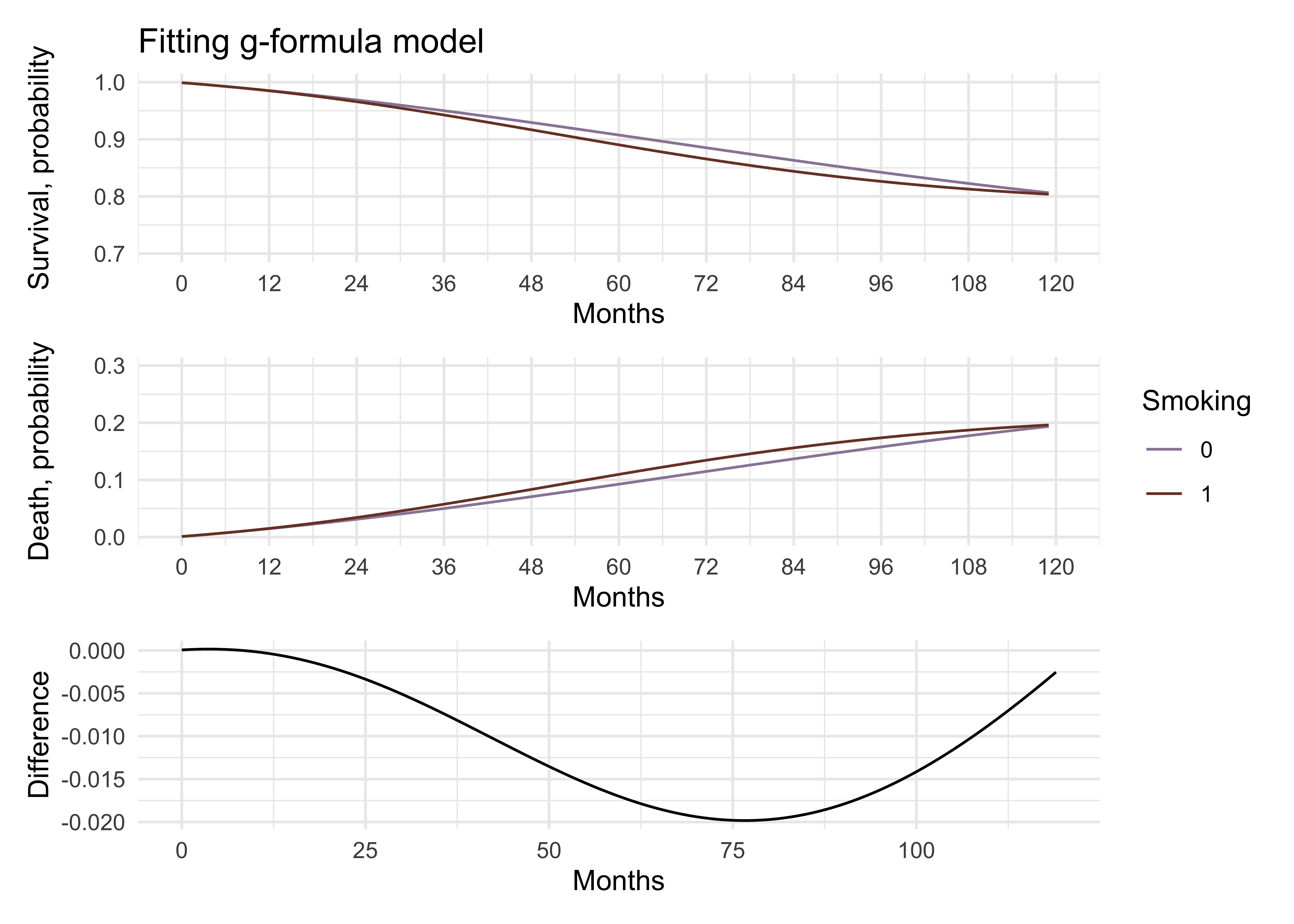
# plot difference
p_gform_3 <- months_gform_mean_diff %>%
  ggplot(aes(x = time, y = p.surv.diff)) +
  geom_line() +
  xlab("Months") + 
  ylab("Difference") + 
  theme_minimal()

# combine plots
p_gform_1 / p_gform_2 / p_gform_3 +
  plot_layout(guides = "collect")

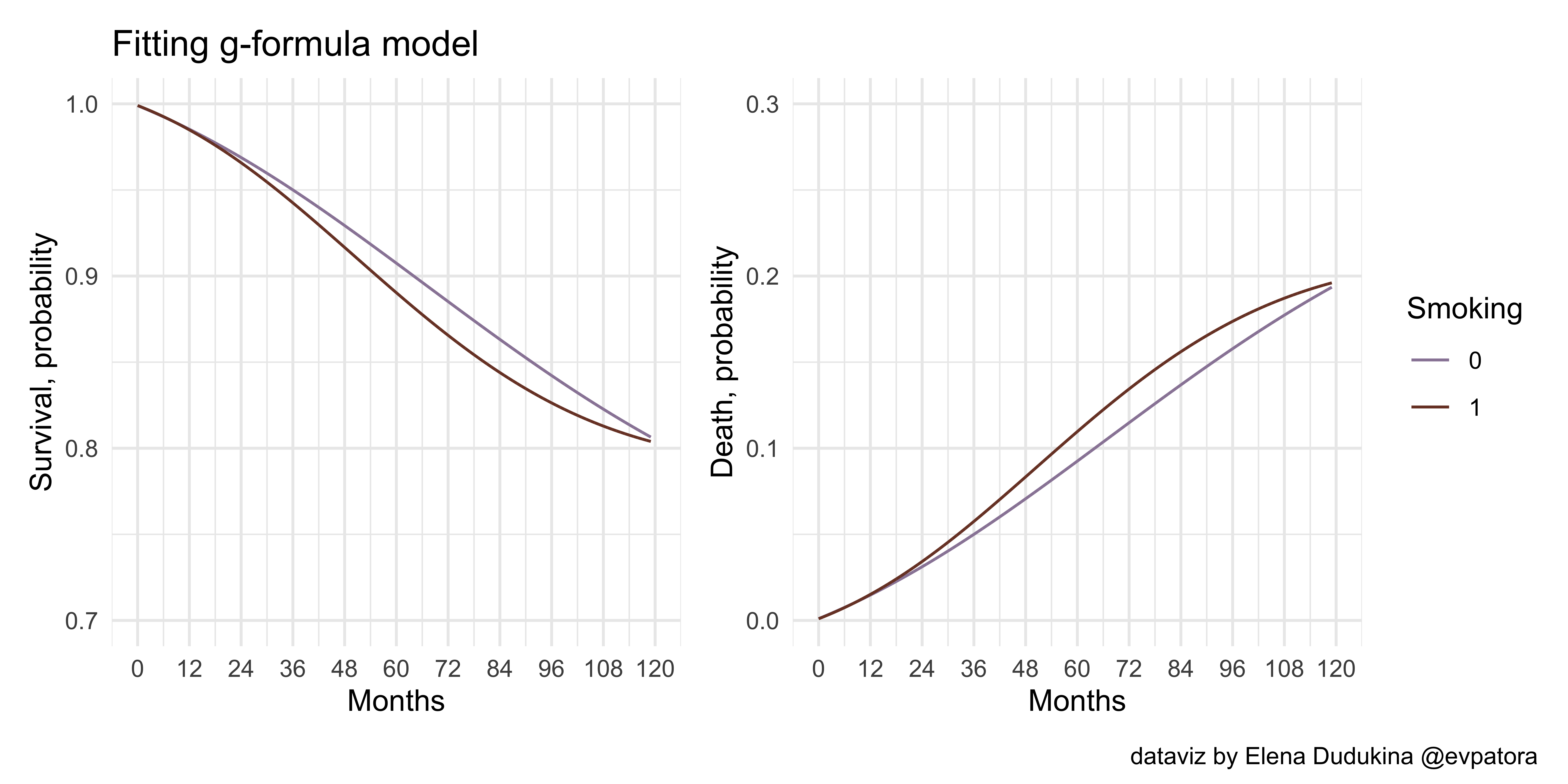
# combine all plots
comb3 <- p_gform_1 + p_gform_2 +
  plot_layout(ncol = 2, guides = "collect") + 
  plot_annotation(
  caption = "dataviz by Elena Dudukina @evpatora"
)
comb3

library(tidymodels)

## ── Attaching packages ────────────────────────────────────── tidymodels 0.1.2 ──

## ✓ broom     0.7.2      ✓ recipes   0.1.15
## ✓ dials     0.0.9      ✓ rsample   0.0.8 
## ✓ infer     0.5.3      ✓ tune      0.1.2 
## ✓ modeldata 0.1.0      ✓ workflows 0.2.1 
## ✓ parsnip   0.1.4      ✓ yardstick 0.0.7

times <- 100

# reduce size of the dataset by keeping only relevant vars
data %<>% select(seqn, survtime, death, qsmk, age, sex, race, education, smokeintensity, smkintensity82_71, smokeyrs, exercise, active, wt71)

set.seed(123456789)
boots <- bootstraps(data, times = times, apparent = FALSE)

# mutate seqn: original + n of repeat
boots %<>% mutate(
  splits = map(splits, ~ as_tibble(.x)),
  splits = map(splits, ~ group_by(.x, seqn) %>% 
                               mutate(rep = row_number()) %>% 
                               ungroup() %>% 
                               mutate(
                                 seqn = paste0(seqn, rep)
                               ))
)

months_gform_list <- map(boots$splits, ~ uncount(.x, weights = survtime, .remove = F) %>% 
  group_by(seqn) %>% 
  mutate (
    time = row_number() - 1,
    event = case_when(
      time == survtime - 1 & death == 1 ~ 1,
      TRUE ~ 0
    ),
    timesq = time*time
  ) %>% 
  ungroup()
  )

# Q-model function
gform_model <- function(data) {
  glm(formula = event == 0 ~ qsmk + I(qsmk*time) + I(qsmk*timesq) + time + timesq + sex + race + age + I(age*age) + as.factor(education) + smokeintensity + I(smokeintensity*smokeintensity) + smkintensity82_71 + smokeyrs + I(smokeyrs*smokeyrs) + as.factor(exercise) + as.factor(active) + wt71 + I(wt71*wt71), family = binomial(link = "logit"), data = data)
  }

# apply gform_model function to all re-sampled datasets
boot_models <- boots %>% 
  mutate(model = map(months_gform_list, ~gform_model(data = .x)))

# compute the P.O.s in each re-sampled long dataset
# create a function, which performs all the steps as in code chunk above with the possibility to set the smoking level
set_qsmk <- function(data, qsmk_level){
  data %<>%  
  mutate(uncount = max(survtime)) %>% 
  # use the same censoring time point of 120 months for all individuals
  uncount(weights = uncount, .remove = T) %>% 
  group_by(seqn) %>% 
  mutate (
    qsmk = qsmk_level, # set exposure level
    time = row_number() - 1,
    event = case_when(
      time == survtime -1 & death == 1 ~ 1,
      TRUE ~ 0
    ),
    timesq = time*time
  ) %>% 
  ungroup() %>% 
  select(seqn, qsmk, time, timesq, age, sex, race, education, smokeintensity, smkintensity82_71, smokeyrs, exercise, active, wt71, event) %>%  
  mutate(
    p.not.event = predict(q_model, type = "response", newdata = .)
  ) %>% 
  group_by(seqn) %>% 
  # compute probability of survival for each individual over all time points
  mutate(p.surv = cumprod(p.not.event)) %>% 
  ungroup()
}

# set exposure to 0
months0_gform_list <- map(.x = boots$splits, ~set_qsmk(data = .x, qsmk_level = 0))

# predict P.O.s
months0_gform_list <- map2(.x = months0_gform_list, .y = boot_models$model, ~  mutate(.x ,
             p.not.event = predict(.y, type = "response", newdata = .x)
  ) %>% 
  group_by(seqn) %>% 
  # compute probability of survival for each individual over all time points
  mutate(p.surv = cumprod(p.not.event)) %>% 
  ungroup()
  )

# list: every observation-month with the assigned exposure level = 1
# exposed
# set exposure to 1
months1_gform_list <- map(.x = boots$splits, ~set_qsmk(data = .x, qsmk_level = 1))

# predict P.O.s
months1_gform_list <- map2(.x = months1_gform_list, .y = boot_models$model, ~ mutate(.x ,
             p.not.event = predict(.y, type = "response", newdata = .x)
  ) %>% 
  group_by(seqn) %>% 
  # compute probability of survival for each individual over all time points
  mutate(p.surv = cumprod(p.not.event)) %>% 
  ungroup())

# compute average survival over each observation-month in each dataset (under exposure and no exposure) and combine
# unexposed
months0_gform_list %<>% 
  map(.x = ., ~ select(.x, seqn, qsmk, time, p.surv) %>% 
        group_by(time) %>% 
        # mean surv
        mutate(p.surv.mean = mean(p.surv)) %>% 
        ungroup() %>% 
        select(time, qsmk, p.surv.mean) %>% 
        distinct()
      )

# exposed
months1_gform_list %<>% 
  map(.x = ., ~ select(.x, seqn, qsmk, time, p.surv) %>% 
        group_by(time) %>% 
        # mean surv
        mutate(p.surv.mean = mean(p.surv)) %>% 
        ungroup() %>% 
        select(time, qsmk, p.surv.mean) %>% 
        distinct()
  )

# difference in survival in each observation month
surv_diff_gform_list <- map(list(months0_gform_list, months1_gform_list), ~bind_rows(., .id = "iteration"))

surv_diff_gform <- surv_diff_gform_list %>% bind_cols(.) %>% 
  mutate(
    surv_diff_gform = p.surv.mean...8 - p.surv.mean...4,
    iteration...1 = as.numeric(iteration...1)
  )

## New names:
## * iteration -> iteration...1
## * time -> time...2
## * qsmk -> qsmk...3
## * p.surv.mean -> p.surv.mean...4
## * iteration -> iteration...5
## * ...

surv_diff_gform %<>% 
  group_by(time...2) %>% 
  summarise_at(.vars = vars(surv_diff_gform), .funs = list(Q2.5 = ~ quantile(., probs = 0.025), Q50 = ~ quantile(., probs = 0.50), Q97.5 = ~ quantile(., probs = 0.975)))

# combine and plot
surv_diff_gform_plot <- surv_diff_gform_list %>% bind_rows(., .id = "id")

surv_diff_gform_plot %<>% 
  group_by(qsmk, time) %>% 
  summarise_at(.vars = vars(p.surv.mean), .funs = list(Q2.5 = ~ quantile(., probs = 0.025), Q50 = ~ quantile(., probs = 0.50), Q97.5 = ~ quantile(., probs = 0.975)))

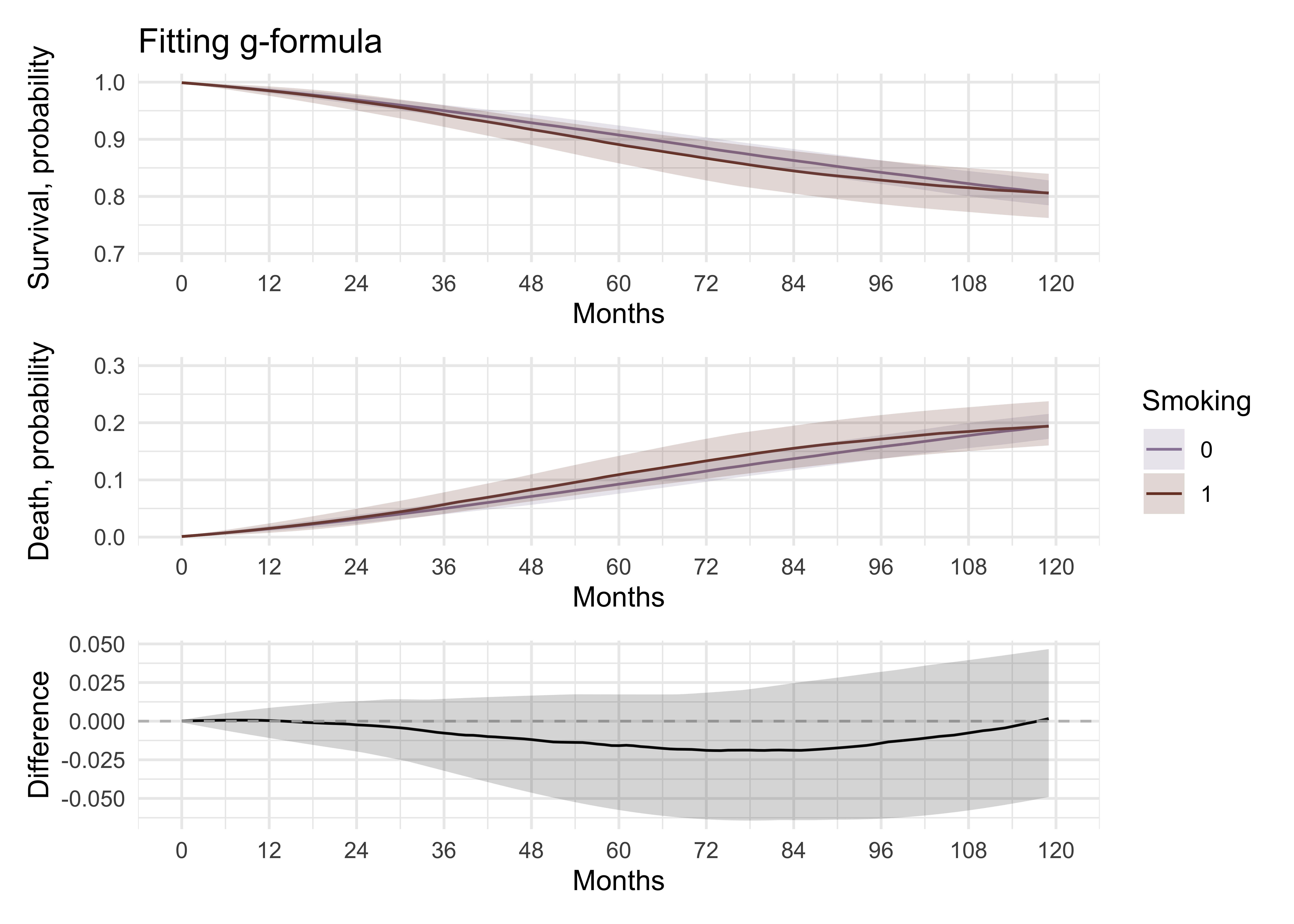
# survival gform with 95% CIs
p_gform_1 <- surv_diff_gform_plot %>% 
  group_by(qsmk) %>% 
  ggplot(aes(x = time, y = Q50, color = factor(qsmk), fill = factor(qsmk))) +
  geom_line() +
  geom_ribbon(aes(ymin = Q2.5, ymax = Q97.5),
              alpha = .2, colour = NA) +
  xlab("Months") + 
  scale_x_continuous(limits = c(0, 120), breaks = seq(0,120,12)) +
  scale_y_continuous(limits = c(0.7, 1), breaks = seq(0.7, 1, 0.1)) +
  ylab("Survival, probability") + 
  ggtitle("Fitting g-formula") +
  theme_minimal()+
  labs(colour = "Smoking", fill = "Smoking") +
  scale_fill_manual(values = wes_palette("IsleofDogs1")) +
  scale_color_manual(values = wes_palette("IsleofDogs1"))

# 1-survival
p_gform_2 <- surv_diff_gform_plot %>% 
  group_by(qsmk) %>% 
  ggplot(aes(x = time, y = 1 - Q50, color = factor(qsmk), fill = factor(qsmk))) +
  geom_line() +
  geom_ribbon(aes(ymin = 1 - Q97.5, ymax = 1 - Q2.5), alpha = .2, colour = NA) +
  scale_x_continuous(limits = c(0, 120), breaks = seq(0, 120, 12)) +
  scale_y_continuous(limits = c(0, 0.3), breaks = seq(0, 0.3, 0.1)) +
  xlab("Months") + 
  ylab("Death, probability") + 
  theme_minimal()+
  labs(colour = "Smoking", fill = "Smoking") +
  scale_fill_manual(values = wes_palette("IsleofDogs1")) +
  scale_color_manual(values = wes_palette("IsleofDogs1"))

p_gform_3 <- surv_diff_gform %>% 
  ggplot(aes(x = time...2, y = Q50)) +
  geom_line() +
  geom_hline(yintercept = 0, color = "grey", linetype = 2) + 
  geom_ribbon(aes(ymin = Q2.5, ymax = Q97.5), alpha = .2, colour = NA) +
  scale_x_continuous(limits = c(0, 120), breaks = seq(0, 120, 12)) +
  xlab("Months") + 
  ylab("Difference") +
  theme_minimal()+
  labs(colour = "Smoking", fill = "Smoking")

# combine gform plots
p_gform_1 / p_gform_2 / p_gform_3 +
  plot_layout(guides = "collect")

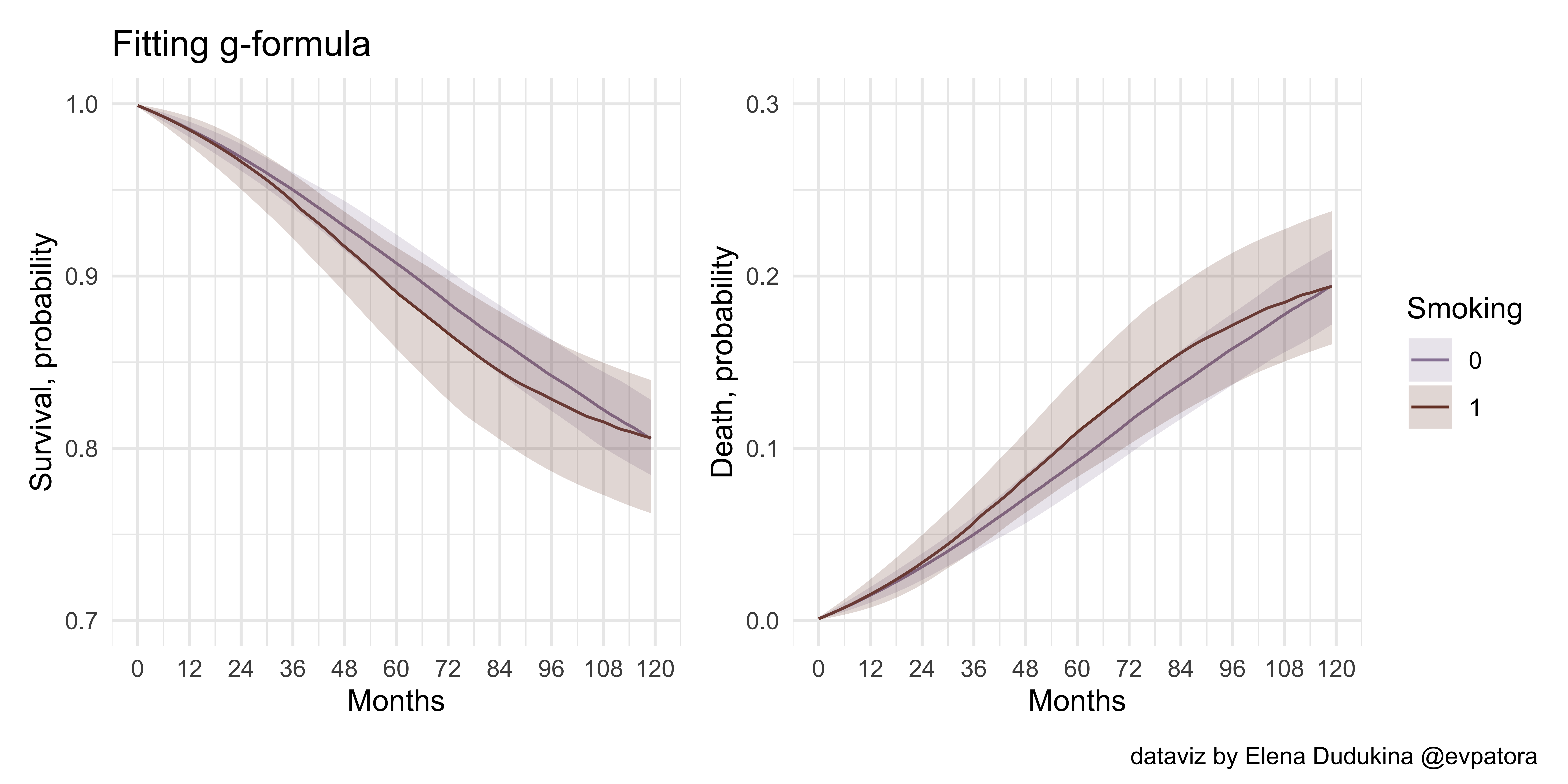
# combine plots
comb4 <- p_gform_1 + p_gform_2 +
  plot_layout(ncol = 2, guides = "collect") + 
  plot_annotation(
  caption = "dataviz by Elena Dudukina @evpatora"
)

comb4

Final notes

As in previous post, I want to stress that causal research question, causal diagram incorporating the assumed data-generating mechanism, and consideration of causal assumptions are pivotal for causal analysis ✌️