Direction of Bias From Nondifferential Misclassification
In this post, I simulate 3 scenarios of non-differential classifications of exposure as demonstrated in Yland et al., 2022:
- Specificity of exposure 90% and sensitivity 60%
- Specificity of exposure 90% and sensitivity 70%
- Specificity of exposure 90% and sensitivity 80%
Each of these scenarios will be simulated in 10 thousand datasets of varying sizes: n=100, n=1000, n=10000.
The aim of this exercise is to demonstrate the deviation from expected direction of bias when non-differential misclassification of exposure is present. The expected direction of bias en non-differential misclassification of exposure is present is towards the null value (dilution); however, in each particular study the bias direction can deviate from the expectation by chance.
Data simulation
To “simulate” a scenario with exact number of exposed and unexposed and to set the “true” risk ratio to 2 (to eliminate randomness), I assign exact counts instead of simulating the data:
# population size size
n1 <- 1e2
n2 <- 1e3
n3 <- 1e4

# data with no misclassification (true scenario): n=100
a1 <- c(rep(0, times = n1))
y1 <- c(rep(0, times = n1))

data1 <- data_frame(a1, y1) %>%
  mutate(
  a1 = case_when(
    row_number() %in% c(1:50) ~ 1,
    T ~ 0
  ),
  y1 = case_when(
    row_number() %in% c(1:10) ~ 1,
    row_number() %in% c(60:64) ~ 1,
    T ~ 0
  )
)
## Warning: `data_frame()` was deprecated in tibble 1.1.0.
## ℹ Please use `tibble()` instead.
## This warning is displayed once every 8 hours.
## Call `lifecycle::last_lifecycle_warnings()` to see where this warning was
## generated.
data1 %>% group_by(a1) %>% count(y1) %>% mutate(p = n/sum(n)*100)
## # A tibble: 4 × 4
## # Groups:   a1 [2]
##      a1    y1     n     p
##   <dbl> <dbl> <int> <dbl>
## 1     0     0    45    90
## 2     0     1     5    10
## 3     1     0    40    80
## 4     1     1    10    20
logbin::logbin(y1~a1, data = data1, method = "em") %>% broom::tidy(exponentiate=T)
## Loading required package: doParallel
## Loading required package: foreach
##
## Attaching package: 'foreach'
## The following objects are masked from 'package:purrr':
##
##     accumulate, when
## Loading required package: iterators
## Loading required package: parallel
## Loading required package: numDeriv
## Loading required package: quantreg
## Loading required package: SparseM
##
## Attaching package: 'SparseM'
## The following object is masked from 'package:base':
##
##     backsolve
##
## Attaching package: 'turboEM'
## The following objects are masked from 'package:numDeriv':
##
##     grad, hessian
## Warning: The `tidy()` method for objects of class `logbin` is not maintained by the broom team, and is only supported through the `glm` tidier method. Please be cautious in interpreting and reporting broom output.
##
## This warning is displayed once per session.
## # A tibble: 2 × 5
##   term        estimate std.error statistic      p.value
##   <chr>          <dbl>     <dbl>     <dbl>        <dbl>
## 1 (Intercept)    0.100     0.424     -5.43 0.0000000572
## 2 a1             2.00      0.510      1.36 0.174
# data with no misclassification (true scenario): n=1000
a2 <- c(rep(0, times = n2))
y2 <- c(rep(0, times = n2))

data2 <- data_frame(a2, y2) %>%
  mutate(
  a2 = case_when(
    row_number() %in% c(1:500) ~ 1,
    T ~ 0
  ),
  y2 = case_when(
    row_number() %in% c(1:100) ~ 1,
    row_number() %in% c(600:649) ~ 1,
    T ~ 0
  )
)

data2 %>% group_by(a2) %>% count(y2) %>% mutate(p = n/sum(n)*100)
## # A tibble: 4 × 4
## # Groups:   a2 [2]
##      a2    y2     n     p
##   <dbl> <dbl> <int> <dbl>
## 1     0     0   450    90
## 2     0     1    50    10
## 3     1     0   400    80
## 4     1     1   100    20
logbin::logbin(y2~a2, data = data2, method = "em") %>% broom::tidy(exponentiate=T)
## # A tibble: 2 × 5
##   term        estimate std.error statistic  p.value
##   <chr>          <dbl>     <dbl>     <dbl>    <dbl>
## 1 (Intercept)    0.100     0.134    -17.2  5.07e-66
## 2 a2             2.00      0.161      4.30 1.72e- 5
# data with no misclassification (true scenario): n=10000
a3 <- c(rep(0, times = n3))
y3 <- c(rep(0, times = n3))

data3 <- data_frame(a3, y3) %>%
  mutate(
  a3 = case_when(
    row_number() %in% c(1:5000) ~ 1,
    T ~ 0
  ),
  y3 = case_when(
    row_number() %in% c(1:1000) ~ 1,
    row_number() %in% c(6000:6499) ~ 1,
    T ~ 0
  )
)

data3 %>% group_by(a3) %>% count(y3) %>% mutate(p = n/sum(n)*100)
## # A tibble: 4 × 4
## # Groups:   a3 [2]
##      a3    y3     n     p
##   <dbl> <dbl> <int> <dbl>
## 1     0     0  4500    90
## 2     0     1   500    10
## 3     1     0  4000    80
## 4     1     1  1000    20
logbin::logbin(y3~a3, data = data3, method = "em") %>% broom::tidy(exponentiate=T)
## # A tibble: 2 × 5
##   term        estimate std.error statistic  p.value
##   <chr>          <dbl>     <dbl>     <dbl>    <dbl>
## 1 (Intercept)    0.100    0.0424     -54.3 0
## 2 a3             2.00     0.0510      13.6 4.36e-42
After we created “true” data without misclassification with varying population sizes, we will set the validity parameters for exposure and observe how non-differential misclassification of exposure and the population size impact the observed risk ratio vs true risk ratio (set to 2-fold increased risk for exposed vs unexposed).
Exposure misclassification: first, set the validity parameters for the simulation. Second, we draw exposure with set validity parametes 10 thousand times for each sensitivity scenario for each populaiton size.
# validity parameters for a
Se1_a = 0.60
Se2_a = 0.70
Se3_a = 0.80
Sp_a = 0.90
FP_a = 1 - Sp_a
# nested data set with 10k rows: facilitating 10k simulation iterations
boots1 <- tibble(
id = c(1:1e4),
splits = list(tibble(data1))
)
# sim a*, n=100
set.seed(398347947)
boots1 %<>% mutate(
splits = map(splits, ~mutate(.x,
astar1 = rbinom(n = n1, size = 1, prob = FP_a + (Se1_a - FP_a) * a1),
astar2 = rbinom(n = n1, size = 1, prob = FP_a + (Se2_a - FP_a) * a1),
astar3 = rbinom(n = n1, size = 1, prob = FP_a + (Se3_a - FP_a) * a1)
)),
models_Se1 = map(splits, ~logbin::logbin(y1~astar1, data = .x, method = "em") %>% broom::tidy(exponentiate=T)),
models_Se2 = map(splits, ~logbin::logbin(y1~astar2, data = .x, method = "em") %>% broom::tidy(exponentiate=T)),
models_Se3 = map(splits, ~logbin::logbin(y1~astar3, data = .x, method = "em") %>% broom::tidy(exponentiate=T)),
astar1res = map(models_Se1, ~filter(.x, term == "astar1") %>% select(estimate)),
astar2res = map(models_Se2, ~filter(.x, term == "astar2") %>% select(estimate)),
astar3res = map(models_Se3, ~filter(.x, term == "astar3") %>% select(estimate))
)
ggplot1 <- boots1 %>% unnest(astar1res) %>%
ggplot(aes(y = estimate)) +
coord_flip() +
geom_density() +
geom_hline(yintercept = 2) +
theme_minimal() +
labs(title = "Sp=0.9, Se=0.6, n=100")
ggplot2 <- boots1 %>% unnest(astar2res) %>%
ggplot(aes(y = estimate)) +
coord_flip() +
geom_density() +
geom_hline(yintercept = 2) +
theme_minimal() +
labs(title = "Sp=0.9, Se=0.7, n=100")
ggplot3 <- boots1 %>% unnest(astar3res) %>%
ggplot(aes(y = estimate)) +
coord_flip() +
geom_density() +
geom_hline(yintercept = 2) +
theme_minimal() +
labs(title = "Sp=0.9, Se=0.8, n=100")
ggplot <- boots1 %>% unnest(cols = c(astar1res, astar2res, astar3res), names_repair = "universal") %>%
pivot_longer(cols = contains("estimate"), names_to = c("simulation_id"), values_to = "estimate") %>%
mutate(
simulation_id = case_when(
simulation_id == "estimate...6" ~ "Sp=0.9, Se=0.6, n=100",
simulation_id == "estimate...7" ~ "Sp=0.9, Se=0.7, n=100",
simulation_id == "estimate...8" ~ "Sp=0.9, Se=0.8, n=100"
)
) %>%
ggplot(aes(y = estimate, color = simulation_id, fill = simulation_id)) +
coord_flip() +
geom_density(alpha=0.2) +
geom_hline(yintercept = 2, color = "darkgrey") +
theme_minimal() +
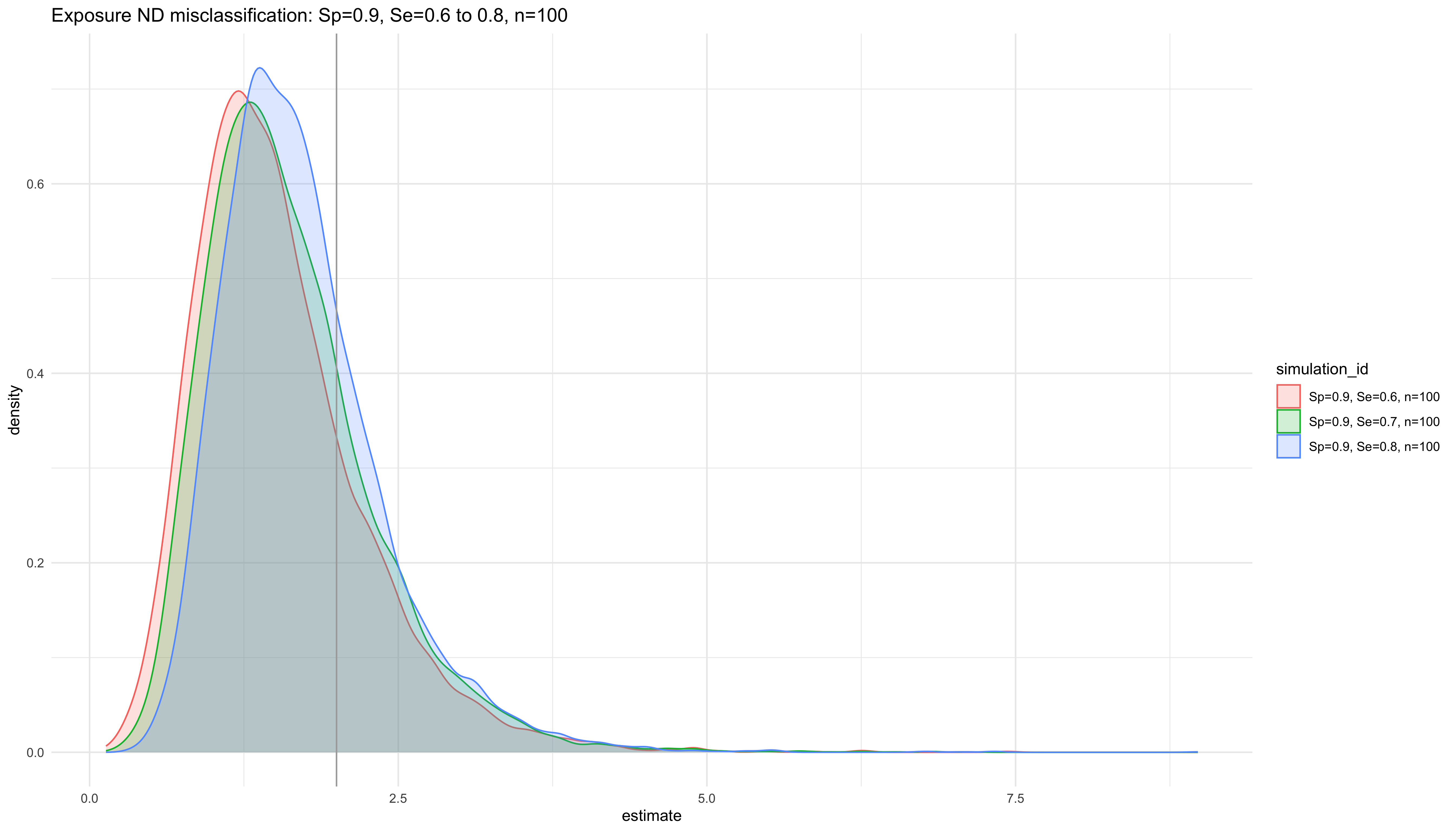
labs(title = "Exposure ND misclassification: Sp=0.9, Se=0.6 to 0.8, n=100")
## New names:
## • `estimate` -> `estimate...6`
## • `estimate` -> `estimate...7`
## • `estimate` -> `estimate...8`
ggsave(ggplot, filename = paste0(Sys.Date(), "-", "n=100", ".pdf"), path = getwd(), device = cairo_pdf,
                                                width = 297, height = 210, units = "mm")

ggplot
# nested data set
boots2 <- tibble(
id = c(1:1e4),
splits = list(tibble(data2))
)
boots2 <- tibble(
id = c(1:1e4),
splits = list(tibble(data2))
)
# sim a*, n=1000
set.seed(398347947)
boots2 %<>% mutate(
splits = map(splits, ~mutate(.x,
astar1 = rbinom(n = n2, size = 1, prob = FP_a + (Se1_a - FP_a) * a2),
astar2 = rbinom(n = n2, size = 1, prob = FP_a + (Se2_a - FP_a) * a2),
astar3 = rbinom(n = n2, size = 1, prob = FP_a + (Se3_a - FP_a) * a2)
)),
models_Se1 = map(splits, ~logbin::logbin(y2~astar1, data = .x, method = "em") %>% broom::tidy(exponentiate=T)),
models_Se2 = map(splits, ~logbin::logbin(y2~astar2, data = .x, method = "em") %>% broom::tidy(exponentiate=T)),
models_Se3 = map(splits, ~logbin::logbin(y2~astar3, data = .x, method = "em") %>% broom::tidy(exponentiate=T)),
astar1res = map(models_Se1, ~filter(.x, term == "astar1") %>% select(estimate)),
astar2res = map(models_Se2, ~filter(.x, term == "astar2") %>% select(estimate)),
astar3res = map(models_Se3, ~filter(.x, term == "astar3") %>% select(estimate))
)
ggplot1 <- boots2 %>% unnest(astar1res) %>%
ggplot(aes(y = estimate)) +
coord_flip() +
geom_density() +
geom_hline(yintercept = 2) +
theme_minimal() +
labs(title = "Sp=0.9, Se=0.6, n=1000")
ggplot2 <- boots2 %>% unnest(astar2res) %>%
ggplot(aes(y = estimate)) +
coord_flip() +
geom_density() +
geom_hline(yintercept = 2) +
theme_minimal() +
labs(title = "Sp=0.9, Se=0.7, n=1000")
ggplot3 <- boots2 %>% unnest(astar3res) %>%
ggplot(aes(y = estimate)) +
coord_flip() +
geom_density() +
geom_hline(yintercept = 2) +
theme_minimal() +
labs(title = "Sp=0.9, Se=0.8, n=1000")
ggplot <- boots2 %>% unnest(cols = c(astar1res, astar2res, astar3res), names_repair = "universal") %>%
pivot_longer(cols = contains("estimate"), names_to = c("simulation_id"), values_to = "estimate") %>%
mutate(
simulation_id = case_when(
simulation_id == "estimate...6" ~ "Sp=0.9, Se=0.6, n=1000",
simulation_id == "estimate...7" ~ "Sp=0.9, Se=0.7, n=1000",
simulation_id == "estimate...8" ~ "Sp=0.9, Se=0.8, n=1000"
)
) %>%
ggplot(aes(y = estimate, color = simulation_id, fill = simulation_id)) +
coord_flip() +
geom_density(alpha=0.2) +
geom_hline(yintercept = 2, color = "darkgrey") +
theme_minimal() +
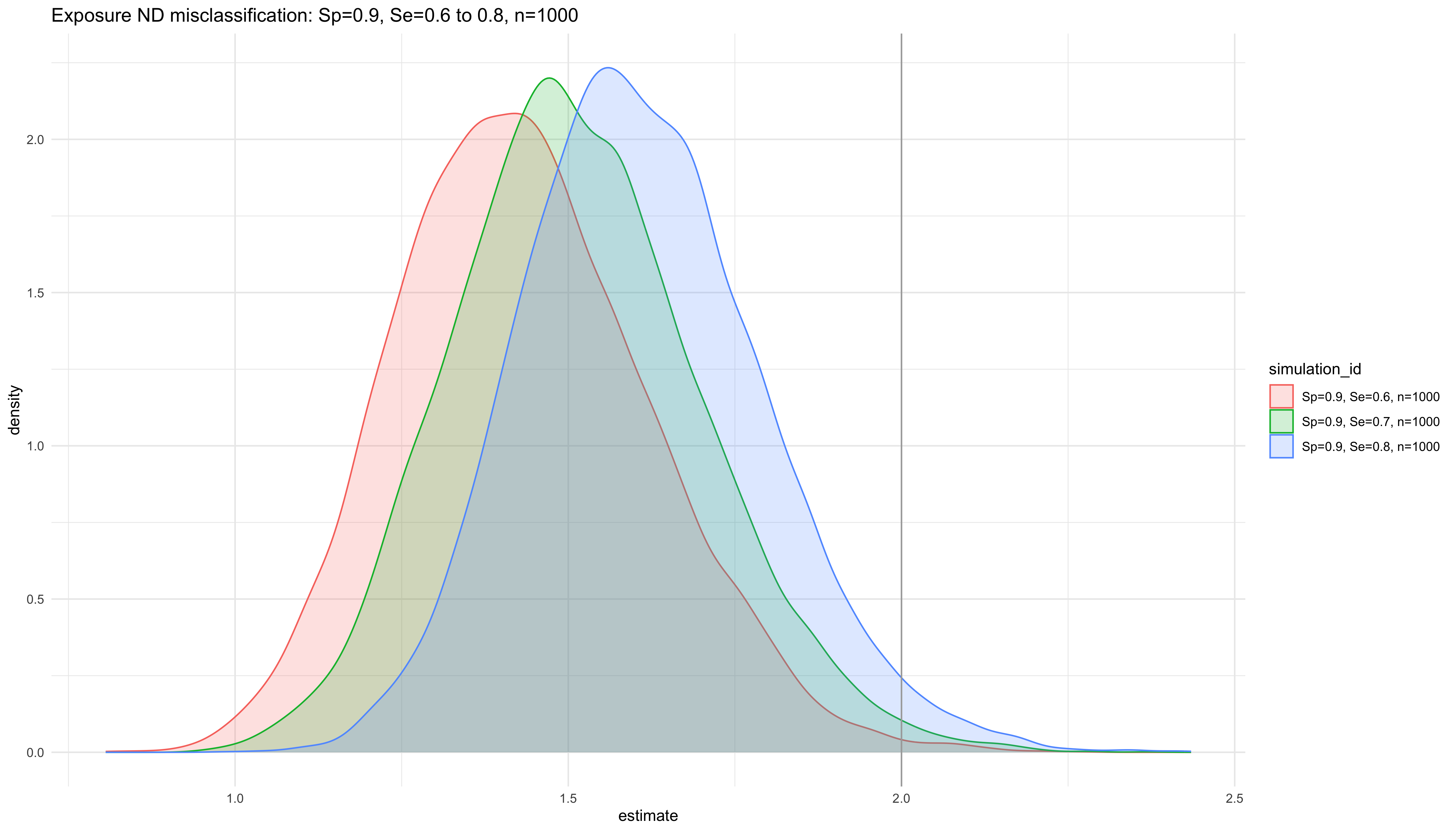
labs(title = "Exposure ND misclassification: Sp=0.9, Se=0.6 to 0.8, n=1000")
## New names:
## • `estimate` -> `estimate...6`
## • `estimate` -> `estimate...7`
## • `estimate` -> `estimate...8`
ggsave(ggplot, filename = paste0(Sys.Date(), "-", "n=1000", ".pdf"), path = getwd(), device = cairo_pdf,
                                                width = 287, height = 200, units = "mm")
ggplot
# nested data set
boots3 <- tibble(
id = c(1:1e4),
splits = list(tibble(data3))
)
# sim a*, n=10000
set.seed(398347947)
boots3 %<>% mutate(
splits = map(splits, ~mutate(.x,
astar1 = rbinom(n = n3, size = 1, prob = FP_a + (Se1_a - FP_a) * a3),
astar2 = rbinom(n = n3, size = 1, prob = FP_a + (Se2_a - FP_a) * a3),
astar3 = rbinom(n = n3, size = 1, prob = FP_a + (Se3_a - FP_a) * a3)
)),
models_Se1 = map(splits, ~logbin::logbin(y3~astar1, data = .x, method = "em") %>% broom::tidy(exponentiate=T)),
models_Se2 = map(splits, ~logbin::logbin(y3~astar2, data = .x, method = "em") %>% broom::tidy(exponentiate=T)),
models_Se3 = map(splits, ~logbin::logbin(y3~astar3, data = .x, method = "em") %>% broom::tidy(exponentiate=T)),
astar1res = map(models_Se1, ~filter(.x, term == "astar1") %>% select(estimate)),
astar2res = map(models_Se2, ~filter(.x, term == "astar2") %>% select(estimate)),
astar3res = map(models_Se3, ~filter(.x, term == "astar3") %>% select(estimate))
)
ggplot1 <- boots3 %>% unnest(astar1res) %>%
ggplot(aes(y = estimate)) +
coord_flip() +
geom_density() +
geom_hline(yintercept = 2) +
theme_minimal() +
labs(title = "Sp=0.9, Se=0.6, n=10000")
ggplot2 <- boots3 %>% unnest(astar2res) %>%
ggplot(aes(y = estimate)) +
coord_flip() +
geom_density() +
geom_hline(yintercept = 2) +
theme_minimal() +
labs(title = "Sp=0.9, Se=0.7, n=10000")
ggplot3 <- boots3 %>% unnest(astar3res) %>%
ggplot(aes(y = estimate)) +
coord_flip() +
geom_density() +
geom_hline(yintercept = 2) +
theme_minimal() +
labs(title = "Sp=0.9, Se=0.8, n=10000")
ggplot <- boots3 %>% unnest(cols = c(astar1res, astar2res, astar3res), names_repair = "universal") %>%
pivot_longer(cols = contains("estimate"), names_to = c("simulation_id"), values_to = "estimate") %>%
mutate(
simulation_id = case_when(
simulation_id == "estimate...6" ~ "Sp=0.9, Se=0.6, n=10000",
simulation_id == "estimate...7" ~ "Sp=0.9, Se=0.7, n=10000",
simulation_id == "estimate...8" ~ "Sp=0.9, Se=0.8, n=10000"
)
) %>%
ggplot(aes(y = estimate, color = simulation_id, fill = simulation_id)) +
coord_flip() +
geom_density(alpha=0.2) +
geom_hline(yintercept = 2, color = "darkgrey") +
theme_minimal() +
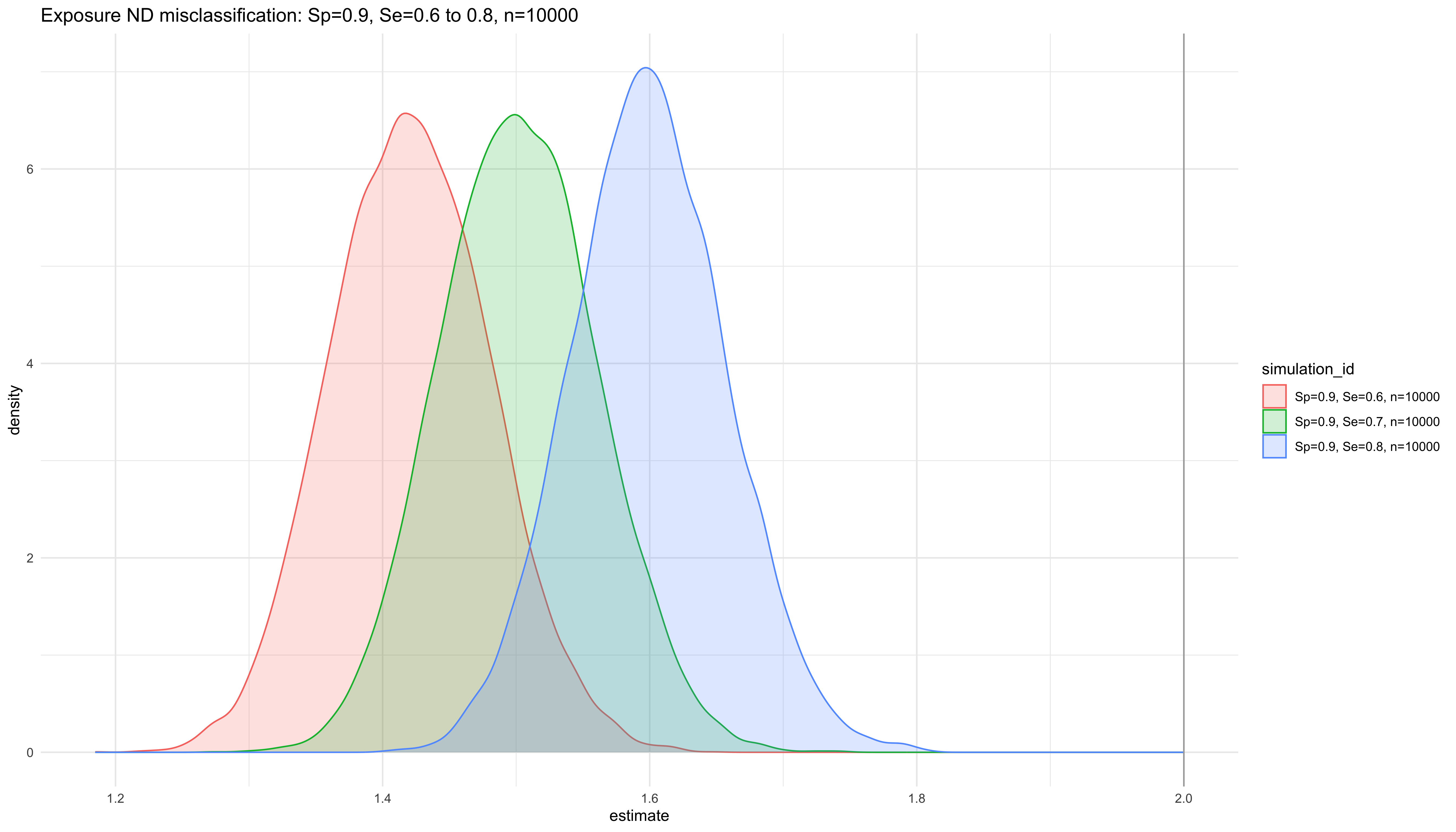
labs(title = "Exposure ND misclassification: Sp=0.9, Se=0.6 to 0.8, n=10000")
## New names:
## • `estimate` -> `estimate...6`
## • `estimate` -> `estimate...7`
## • `estimate` -> `estimate...8`
ggsave(ggplot, filename = paste0(Sys.Date(), "-", "n=10000", ".pdf"), path = getwd(), device = cairo_pdf,
                                                width = 297, height = 210, units = "mm")
ggplot
# Replicate Figure 1 in the paper
boots <- bind_rows(boots1, boots2, boots3) %>%
  mutate(
    `Population size` = case_when(
      row_number() %in% c(1:1e4) ~ "n=100",
      row_number() %in% c(10001:2e4) ~ "n=1000",
      row_number() %in% c(20001:3e4) ~ "n=10000"
    )
  )

ggplot <- boots %>% unnest(cols = c(astar1res, astar2res, astar3res), names_repair = "universal") %>%
  pivot_longer(cols = contains("estimate"), names_to = c("simulation_id"), values_to = "estimate") %>%
  mutate(
    simulation_id = case_when(
      simulation_id == "estimate...6" ~ "Sp=0.9, Se=0.6, n=1e2",
      simulation_id == "estimate...7" ~ "Sp=0.9, Se=0.7, n=1e2",
      simulation_id == "estimate...8" ~ "Sp=0.9, Se=0.8, n=1e2",
      simulation_id == "estimate...9" ~ "Sp=0.9, Se=0.6, n=1e3",
      simulation_id == "estimate...10" ~ "Sp=0.9, Se=0.7, n=1e3",
      simulation_id == "estimate...11" ~ "Sp=0.9, Se=0.8, n=1e3",
      simulation_id == "estimate...12" ~ "Sp=0.9, Se=0.6, n=1e4",
      simulation_id == "estimate...13" ~ "Sp=0.9, Se=0.7, n=1e4",
      simulation_id == "estimate...14" ~ "Sp=0.9, Se=0.8, n=1e4"),

      Se = case_when(
        str_detect(simulation_id, "Se=0.6") ~ "Se=0.6",
        str_detect(simulation_id, "Se=0.7") ~ "Se=0.7",
                   T ~ "Se=0.8")
      ) %>%
  ggplot(aes(y = estimate, color = `Population.size`, fill = `Population.size`)) +
  coord_flip() +
  geom_density(alpha=0.2) +
  geom_hline(yintercept = 2, color = "darkgrey") +
  theme_minimal() +
  facet_wrap(ncol=3, facets = c("Se")) +
  labs(title = "Exposure ND misclassification: Sp=0.9, Se=0.6 to 0.8, Population size: n=1e2, n=1e3, n=1e4", x="Density") +
  annotate(geom = 'richtext', x = 4, y = 6, label = "<i style='color:#D55E00'>*Area of ND misclassification<br>away from the null<br>by chance*</i>", angle = 0)
## New names:
## • `estimate` -> `estimate...6`
## • `estimate` -> `estimate...7`
## • `estimate` -> `estimate...8`
## • `Population size` -> `Population.size`
ggsave(ggplot, filename = paste0(Sys.Date(), "-Figure 1", ".pdf"), path = getwd(), device = cairo_pdf,
                                                width = 297, height = 210, units = "mm")
ggplot
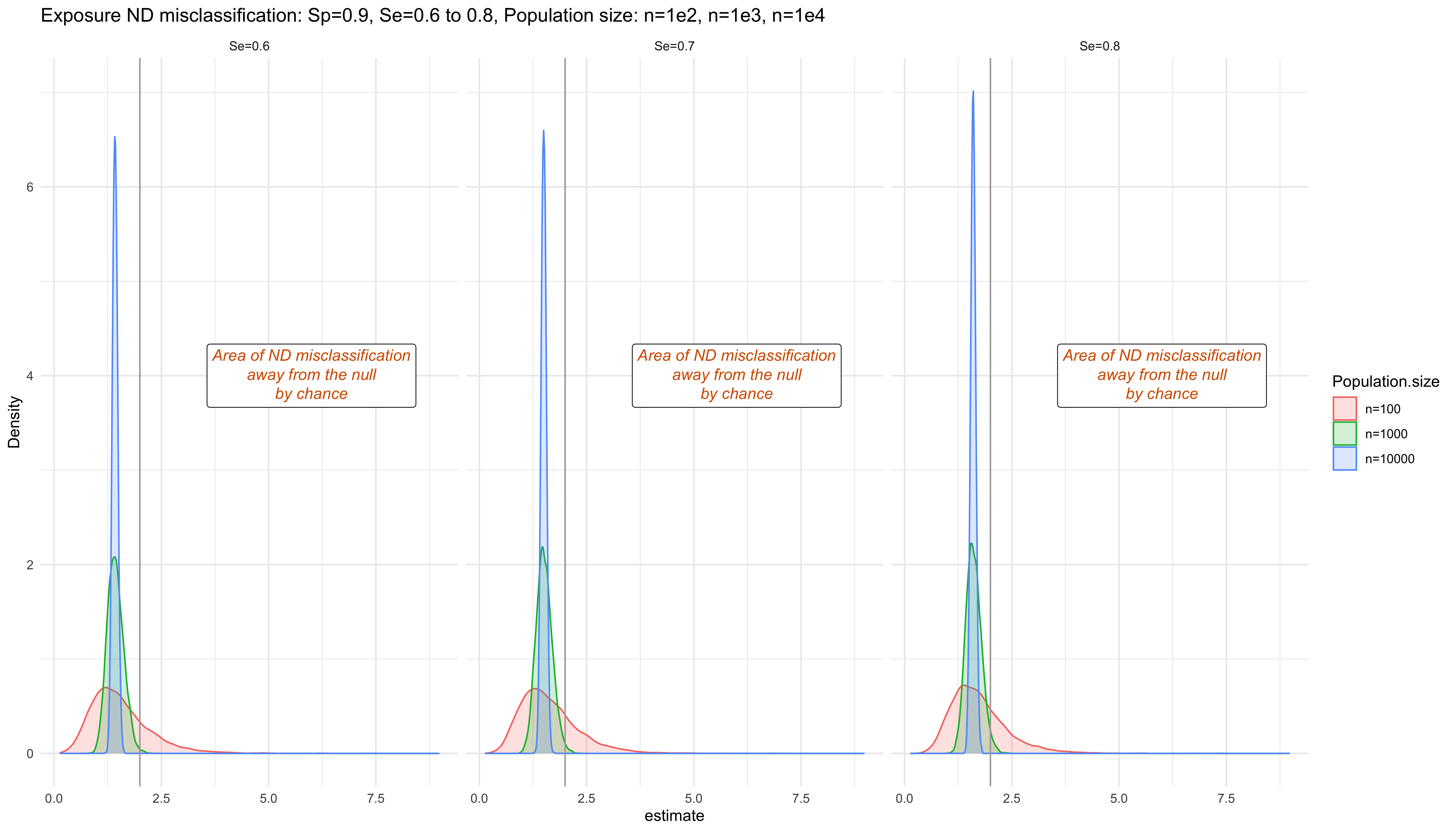
Conclusions
- Smaller sample size and scenarios with less misclassification are more likely to be biased away from the null due to chance.
- Non-differential misclassification is expected to bias the results towards the null (dilution of the true measure of effect), however, each particular study results may be biased away from the null value due to chance.
References
- Yland JJ, Wesselink AK, Lash TL, Fox MP. Misconceptions About the Direction of Bias From Nondifferential Misclassification. American Journal of Epidemiology. 2022;191(8):1485-1495. doi:https://doi.org/10.1093/aje/kwac035