Antibiotics utilization in Denmark: using R to solve practical tasks in epidemiology
R-Ladies Abuja 2022
Intro
This is a blog post-chaperon for the R-Ladies meet-up Abuja. We are talking R in epidemiology, practical aspects of being R-user and going through data-supported example of how to use R for data aggregation and visualization.
Getting started
library(tidyverse)
library(magrittr)
library(wesanderson)
First things first - downloading data. You can also find a full instruction here and here
link_list_dk <- list(
  "1996_atc_code_data.txt" = "https://medstat.dk/da/download/file/MTk5Nl9hdGNfY29kZV9kYXRhLnR4dA==",
  "1997_atc_code_data.txt"  = "https://medstat.dk/da/download/file/MTk5N19hdGNfY29kZV9kYXRhLnR4dA==",
  "1998_atc_code_data.txt" = "https://medstat.dk/da/download/file/MTk5OF9hdGNfY29kZV9kYXRhLnR4dA==",
  "1999_atc_code_data.txt" = "https://medstat.dk/da/download/file/MTk5OV9hdGNfY29kZV9kYXRhLnR4dA==",
  "2000_atc_code_data.txt" = "https://medstat.dk/da/download/file/MjAwMF9hdGNfY29kZV9kYXRhLnR4dA==",
  "2001_atc_code_data.txt" = "https://medstat.dk/da/download/file/MjAwMV9hdGNfY29kZV9kYXRhLnR4dA==",
  "2002_atc_code_data.txt" = "https://medstat.dk/da/download/file/MjAwMl9hdGNfY29kZV9kYXRhLnR4dA==",
  "2003_atc_code_data.txt" = "https://medstat.dk/da/download/file/MjAwM19hdGNfY29kZV9kYXRhLnR4dA==",
  "2004_atc_code_data.txt" = "https://medstat.dk/da/download/file/MjAwNF9hdGNfY29kZV9kYXRhLnR4dA==",
  "2006_atc_code_data.txt" = "https://medstat.dk/da/download/file/MjAwNl9hdGNfY29kZV9kYXRhLnR4dA==",
  "2007_atc_code_data.txt" = "https://medstat.dk/da/download/file/MjAwN19hdGNfY29kZV9kYXRhLnR4dA==",
  "2008_atc_code_data.txt" = "https://medstat.dk/da/download/file/MjAwOF9hdGNfY29kZV9kYXRhLnR4dA==",
  "2009_atc_code_data.txt" = "https://medstat.dk/da/download/file/MjAwOV9hdGNfY29kZV9kYXRhLnR4dA==",
  "2010_atc_code_data.txt" = "https://medstat.dk/da/download/file/MjAxMF9hdGNfY29kZV9kYXRhLnR4dA==",
  "2011_atc_code_data.txt" = "https://medstat.dk/da/download/file/MjAxMV9hdGNfY29kZV9kYXRhLnR4dA==",
  "2012_atc_code_data.txt" = "https://medstat.dk/da/download/file/MjAxMl9hdGNfY29kZV9kYXRhLnR4dA==",
  "2013_atc_code_data.txt" = "https://medstat.dk/da/download/file/MjAxM19hdGNfY29kZV9kYXRhLnR4dA==",
  "2014_atc_code_data.txt" = "https://medstat.dk/da/download/file/MjAxNF9hdGNfY29kZV9kYXRhLnR4dA==",
  "2015_atc_code_data.txt" = "https://medstat.dk/da/download/file/MjAxNV9hdGNfY29kZV9kYXRhLnR4dA==",
  "2016_atc_code_data.txt" = "https://medstat.dk/da/download/file/MjAxNl9hdGNfY29kZV9kYXRhLnR4dA==",
  "2017_atc_code_data.txt" = "https://medstat.dk/da/download/file/MjAxN19hdGNfY29kZV9kYXRhLnR4dA==",
  "2018_atc_code_data.txt" = "https://medstat.dk/da/download/file/MjAxOF9hdGNfY29kZV9kYXRhLnR4dA==",
  "2019_atc_code_data.txt" = "https://medstat.dk/da/download/file/MjAxOV9hdGNfY29kZV9kYXRhLnR4dA==",
  "2020_atc_code_data.txt" = "https://medstat.dk/da/download/file/MjAyMF9hdGNfY29kZV9kYXRhLnR4dA==",
  "atc_code_text.txt" = "https://medstat.dk/da/download/file/YXRjX2NvZGVfdGV4dC50eHQ=",
  "atc_groups.txt" = "https://medstat.dk/da/download/file/YXRjX2dyb3Vwcy50eHQ=",
  "population_data.txt" = "https://medstat.dk/da/download/file/cG9wdWxhdGlvbl9kYXRhLnR4dA=="
)

# ATC codes are stored in files
seq_atc <- c(1:24)
atc_code_data_list <- link_list_dk[seq_atc]

# drugs names
eng_drug <- read_delim(link_list_dk[["atc_groups.txt"]], delim = ";", col_names = c(paste0("V", c(1:6))), col_types = cols(V1 = col_character(), V2 = col_character(), V3 = col_character(), V4 = col_character(), V5 = col_character(), V6 = col_character())) %>%
  # keep drug classes labels in English
  filter(V5 == "1") %>%
  select(ATC = V1,
         drug = V2,
         unit_dk = V4)

# drugs data
atc_data <- map(atc_code_data_list, ~read_delim(file = .x, delim = ";", trim_ws = T, col_names = c(paste0("V", c(1:14))), col_types = cols(V1 = col_character(), V2 = col_character(), V3 = col_character(), V4 = col_character(), V5 = col_character(),V6 = col_character(), V7 = col_character(), V8 = col_character(), V9 = col_character(), V10 = col_character(), V11 = col_character(), V12 = col_character(), V13 = col_character(), V14 = col_character()))) %>%
  # bind atc_data from all years
  bind_rows()

# population data
pop_data <- read_delim(link_list_dk[["population_data.txt"]], delim = ";", col_names = c(paste0("V", c(1:7))), col_types = cols(V1 = col_character(), V2 = col_character(), V3 = col_character(), V4 = col_character(), V5 = col_character(), V6 = col_character(), V7 = col_character())) %>%
  # rename and keep columns
  select(year = V1,
         region_text = V2,
         region = V3,
         gender = V4,
         age = V5,
         denominator_per_year = V6) %>%
  # human-reading friendly label on sex categories
  mutate(
      gender_text = case_when(
      gender == "1" ~ "men",
      gender == "2" ~ "women",
      T ~ as.character(gender)
    )
  ) %>%
  # make numeric variables
  mutate_at(vars(year, age, denominator_per_year), as.numeric) %>%
  arrange(year, age, region, gender)
Explore data structure
atc_data %>% skimr::skim()
| Name | Piped data |
| Number of rows | 28814496 |
| Number of columns | 14 |
| _______________________ | |
| Column type frequency: | |
| character | 14 |
| ________________________ | |
| Group variables | None |
Table 1: Data summary
Variable type: character
| skim_variable | n_missing | complete_rate | min | max | empty | n_unique | whitespace |
|---|---|---|---|---|---|---|---|
| V1 | 0 | 1.00 | 1 | 7 | 0 | 2967 | 0 |
| V2 | 0 | 1.00 | 4 | 4 | 0 | 24 | 0 |
| V3 | 0 | 1.00 | 1 | 1 | 0 | 3 | 0 |
| V4 | 0 | 1.00 | 1 | 1 | 0 | 6 | 0 |
| V5 | 0 | 1.00 | 1 | 1 | 0 | 4 | 0 |
| V6 | 0 | 1.00 | 1 | 5 | 0 | 104 | 0 |
| V7 | 513229 | 0.98 | 1 | 7 | 0 | 62562 | 0 |
| V8 | 513229 | 0.98 | 1 | 7 | 0 | 86412 | 0 |
| V9 | 186071 | 0.99 | 1 | 8 | 0 | 79983 | 0 |
| V10 | 637631 | 0.98 | 1 | 7 | 0 | 58064 | 0 |
| V11 | 1309019 | 0.95 | 1 | 6 | 0 | 33861 | 0 |
| V12 | 1309167 | 0.95 | 1 | 6 | 0 | 8403 | 0 |
| V13 | 368860 | 0.99 | 1 | 3 | 0 | 101 | 0 |
| V14 | 28814496 | 0.00 | NA | NA | 0 | 0 | 0 |
Clean data
atc_data %<>%
  # rename and keep columns
  rename(
    ATC = V1,
    year = V2,
    sector = V3,
    region = V4,
    gender = V5, # 0 - both; 1 - male; 2 - female; A - age in categories
    age = V6,
    number_of_people = V7,
    patients_per_1000_inhabitants = V8,
    turnover = V9,
    regional_grant_paid = V10,
    quantity_sold_1000_units = V11,
    quantity_sold_units_per_unit_1000_inhabitants_per_day = V12,
    percentage_of_sales_in_the_primary_sector = V13
  )

atc_data %<>%
  # clean columns names and set-up labels
  mutate(
    year = as.numeric(year),
    region_text = case_when(
      region == "0" ~ "DK",
      region == "1" ~ "Region Hovedstaden",
      region == "2" ~ "Region Midtjylland",
      region == "3" ~ "Region Nordjylland",
      region == "4" ~ "Region Sjælland",
      region == "5" ~ "Region Syddanmark",
      T ~ NA_character_
    ),
    gender_text = case_when(
      gender == "0" ~ "both sexes",
      gender == "1" ~ "men",
      gender == "2" ~ "women",
      T ~ as.character(gender)
    )
  ) %>%
  mutate_at(vars(turnover, regional_grant_paid, quantity_sold_1000_units, quantity_sold_units_per_unit_1000_inhabitants_per_day, number_of_people, patients_per_1000_inhabitants), as.numeric) %>%
  select(-V14) %>%
  filter(
  region == "0",
  sector == "0",
  gender != "0"
)

atc_data %<>%
  # deal with non-numeric age in groups
  filter(
    str_detect(age, "[0-9][0-9][0-9]")
  ) %>%
  mutate(
    age = parse_number(age)
  ) %>%
  select(year, ATC, gender, age, number_of_people, patients_per_1000_inhabitants, region_text, gender_text)

atc_data %>% slice(1:100)
## # A tibble: 100 × 8
##     year ATC   gender   age number_of_people patients_per_1000_inha… region_text
##    <dbl> <chr> <chr>  <dbl>            <dbl>                   <dbl> <chr>
##  1  1999 A     2          0             6824                   212.  DK
##  2  1999 A     1          0             7760                   228.  DK
##  3  1999 A     2          1             2633                    79.6 DK
##  4  1999 A     1          1             2872                    82.3 DK
##  5  1999 A     2          2             1049                    31.6 DK
##  6  1999 A     1          2             1132                    32.3 DK
##  7  1999 A     2          3              545                    15.8 DK
##  8  1999 A     1          3              597                    16.4 DK
##  9  1999 A     2          4              412                    11.8 DK
## 10  1999 A     1          4              482                    13.2 DK
## # … with 90 more rows, and 1 more variable: gender_text <chr>
We will examine the utilization of antimicrobials for systemic use by sex and age group and assess temporal trends. For this, we, first, need to specify the groups of codes we are interested in.
Antimictbials for systemic use
regex_AB <- "^J01$"
regex_TETRACYCLINES <- "^J01A$"
regex_AMPHENICOLS <- "^J01B$"
regex_BETALACTAMS <- "^J01C$"
regex_OTHER_BETALACTAMS <- "^J01D$"
regex_SULFONAMIDES_TRIMETHOPRIM <- "^J01E$"
regex_MACROLIDES_LINCOSAMIDES_STREPTOGRAMINS <- "^J01F$"
regex_AMINOGLYCOSIDES <- "^J01G$"
regex_QUINOLONES <- "^J01M$"
# regex_COMB <- "^J01R$"
# regex_OTHER <- "^J01X$"

# combine all ATC codes in one regex string
all_regex <- paste(regex_AB, regex_AB, regex_TETRACYCLINES, regex_AMPHENICOLS, regex_BETALACTAMS, regex_OTHER_BETALACTAMS, regex_SULFONAMIDES_TRIMETHOPRIM, regex_MACROLIDES_LINCOSAMIDES_STREPTOGRAMINS, regex_AMINOGLYCOSIDES, regex_QUINOLONES, sep = "|")
Keep only the ATC codes we are interested in
atc_data %<>% filter(str_detect(ATC, all_regex))
Merge/join with the drugs names dataset
atc_data %<>% left_join(eng_drug)
## Joining, by = "ATC"
Merge/join with the population data
# join with the population data
atc_data %<>% left_join(pop_data)
## Joining, by = c("year", "gender", "age", "region_text", "gender_text")
# create age bands
atc_data %<>% mutate(
  age_cat = cut(age, c(-Inf, 18, 25, 30, 35, 40, 45, 50, 55, 60, 65, 70, Inf))
)

atc_data %>% count(age_cat)
## # A tibble: 12 × 2
##    age_cat       n
##    <fct>     <int>
##  1 (-Inf,18]  5873
##  2 (18,25]    2280
##  3 (25,30]    1613
##  4 (30,35]    1601
##  5 (35,40]    1607
##  6 (40,45]    1583
##  7 (45,50]    1552
##  8 (50,55]    1533
##  9 (55,60]    1534
## 10 (60,65]    1537
## 11 (65,70]    1511
## 12 (70, Inf]  7155
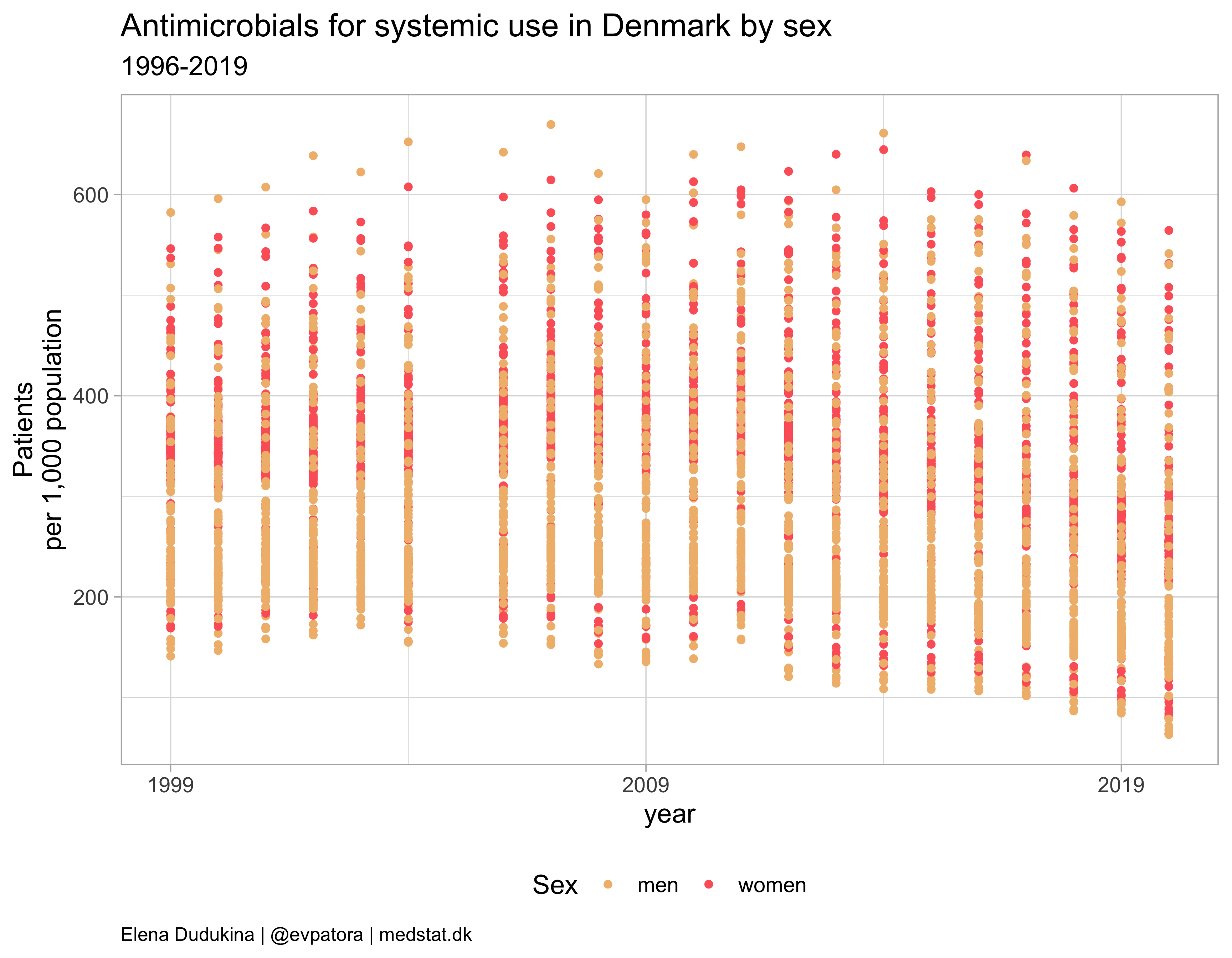
Explore the time trends of overall antibiotics use by sex
atc_data %>%
  filter(str_detect(ATC, regex_AB)) %>%
  ggplot(aes(x = year, y = patients_per_1000_inhabitants, color = gender_text)) +
  geom_point() +
  theme_light(base_size = 14) +
  scale_x_continuous(breaks = c(seq(1999, 2019, 10))) +
  scale_color_manual(values = wes_palette(name = "GrandBudapest1", type = "discrete")) +
  theme(plot.caption = element_text(hjust = 0, size = 10),
        legend.position = "bottom",
        panel.spacing = unit(0.8, "cm")) +
  guides(colour = guide_legend("Sex", ncol = 2)) +
  labs(y = "Patients\nper 1,000 population", title = "Antimicrobials for systemic use in Denmark by sex", subtitle = "1996-2019", caption = "Elena Dudukina | @evpatora | medstat.dk")
What is the problem with the data?
The data is for yearly drug use per age category in 1-year bands, while we need the drug use per wider age category.
# create drug use rates for age categories
atc_data %<>%
  group_by(gender, age_cat, ATC, year) %>%
  mutate(
    numerator = sum(number_of_people),
    denominator = sum(denominator_per_year),
    patients_per_1000_inhabitants = numerator / denominator * 1e3
  ) %>%
  ungroup() %>%
  distinct(gender, age_cat, ATC, year, patients_per_1000_inhabitants, .keep_all = T) %>%
  select(-age)
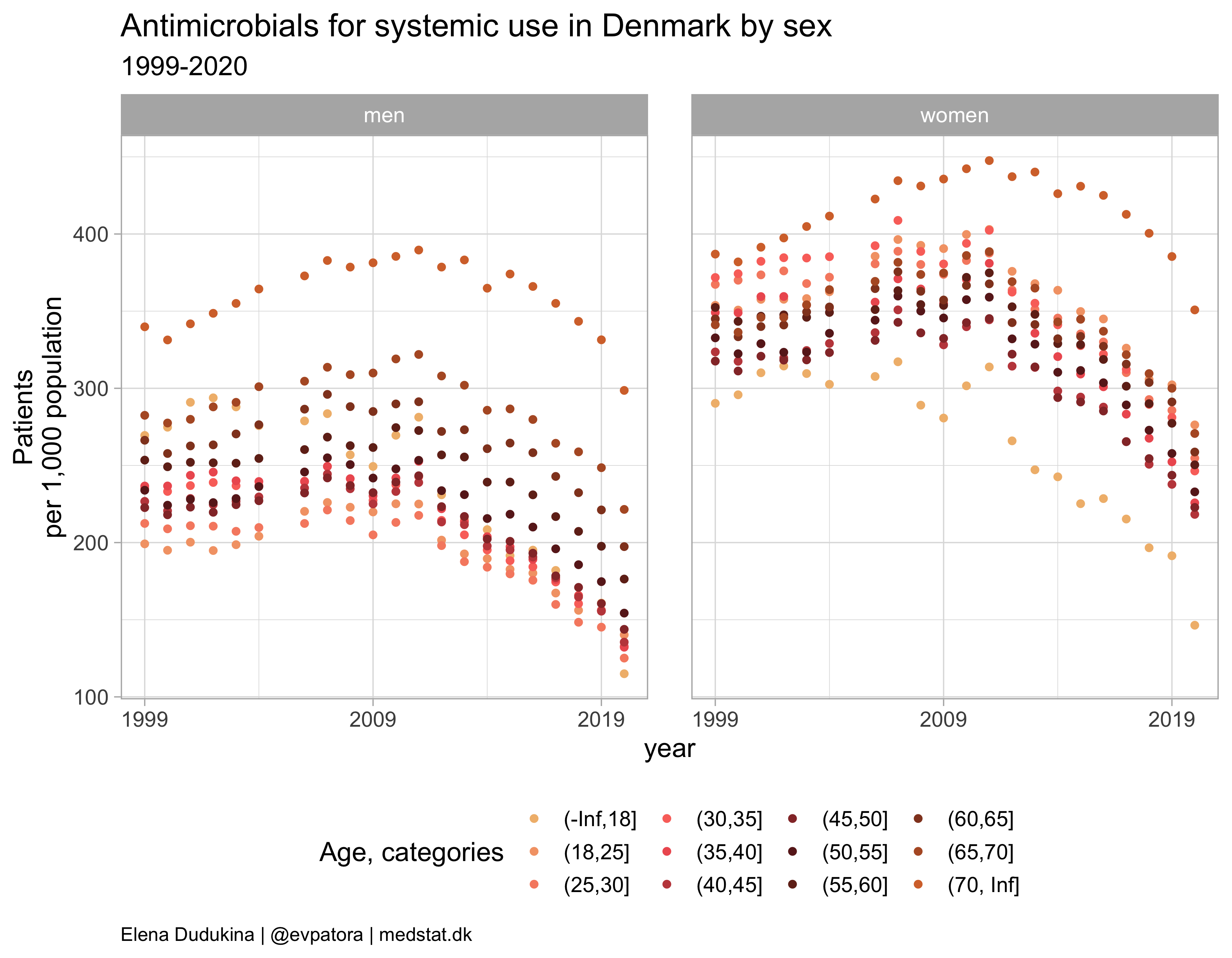
Antibiotics use by year, sex, and age group
atc_data %>%
  filter(str_detect(ATC, regex_AB)) %>%
  ggplot(aes(x = year, y = patients_per_1000_inhabitants, color = age_cat)) +
  geom_point() +
  facet_grid(cols = vars(gender_text)) +
  theme_light(base_size = 14) +
  scale_x_continuous(breaks = c(seq(1999, 2019, 10))) +
  scale_color_manual(values = wes_palette(name = "GrandBudapest1", type = "continuous", n = 12)) +
  theme(plot.caption = element_text(hjust = 0, size = 10),
        legend.position = "bottom",
        panel.spacing = unit(0.8, "cm")) +
  guides(color = guide_legend("Age, categories", ncol = 4)) +
  labs(y = "Patients\nper 1,000 population", title = "Antimicrobials for systemic use in Denmark by sex", subtitle = "1999-2020", caption = "Elena Dudukina | @evpatora | medstat.dk")
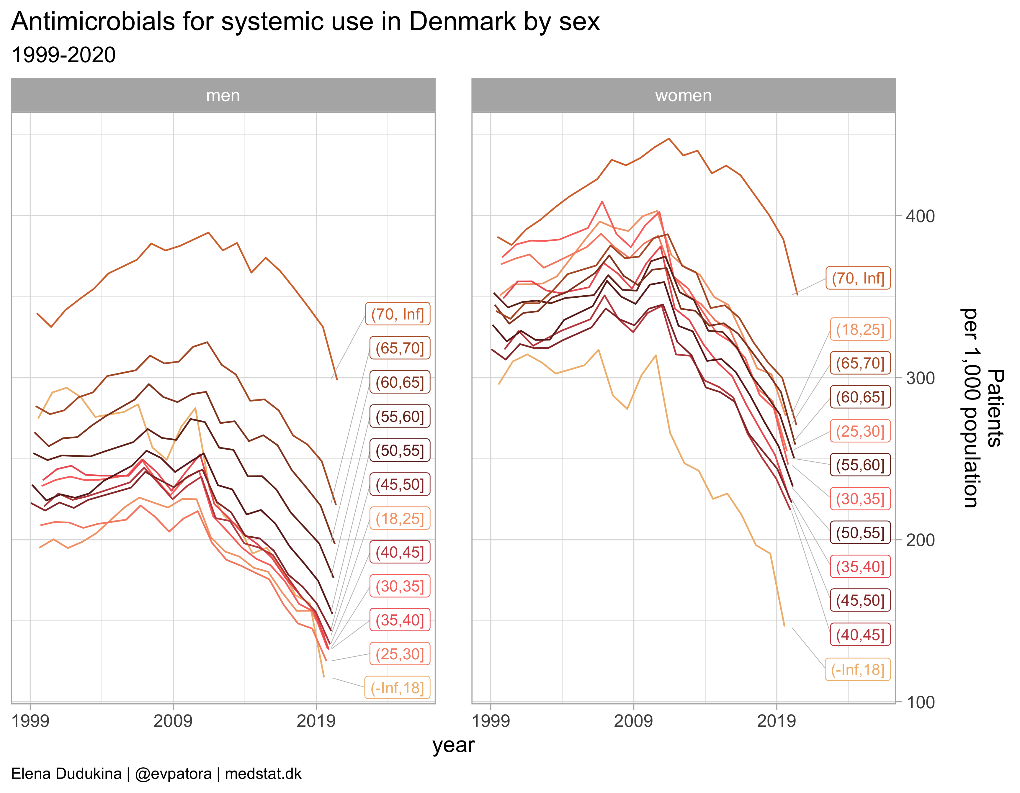
atc_data %>%
  filter(str_detect(ATC, regex_AB)) %>%
  mutate(label = if_else(year == max(year), as.character(age_cat), NA_character_)) %>%
  ggplot(aes(x = year, y = patients_per_1000_inhabitants, color = age_cat)) +
  geom_path(position = position_dodge(width = 1)) +
  facet_grid(cols = vars(gender_text)) +
  theme_light(base_size = 14) +
  scale_x_continuous(limits = c(1999, 2026), breaks = c(seq(1999, 2020, 10))) +
  scale_y_continuous(position = "right") +
  scale_color_manual(values = wes_palette(name = "GrandBudapest1", type = "continuous", n = 12)) +
  theme(plot.caption = element_text(hjust = 0, size = 10),
        legend.position = "none",
        panel.spacing = unit(0.8, "cm")) +
  labs(y = "Patients\nper 1,000 population\n", title = "Antimicrobials for systemic use in Denmark by sex", subtitle = "1999-2020", caption = "Elena Dudukina | @evpatora | medstat.dk") +
  ggrepel::geom_label_repel(aes(label = label, na.rm = TRUE), direction = "y", segment.size = 0.2, segment.colour = "grey", show.legend = F, size = 3.5, nudge_x = 5, hjust = 0.5, max.overlaps = 20)
## Warning: Ignoring unknown aesthetics: na.rm

## Warning: Removed 6 row(s) containing missing values (geom_path).

## Warning: Removed 480 rows containing missing values (geom_label_repel).
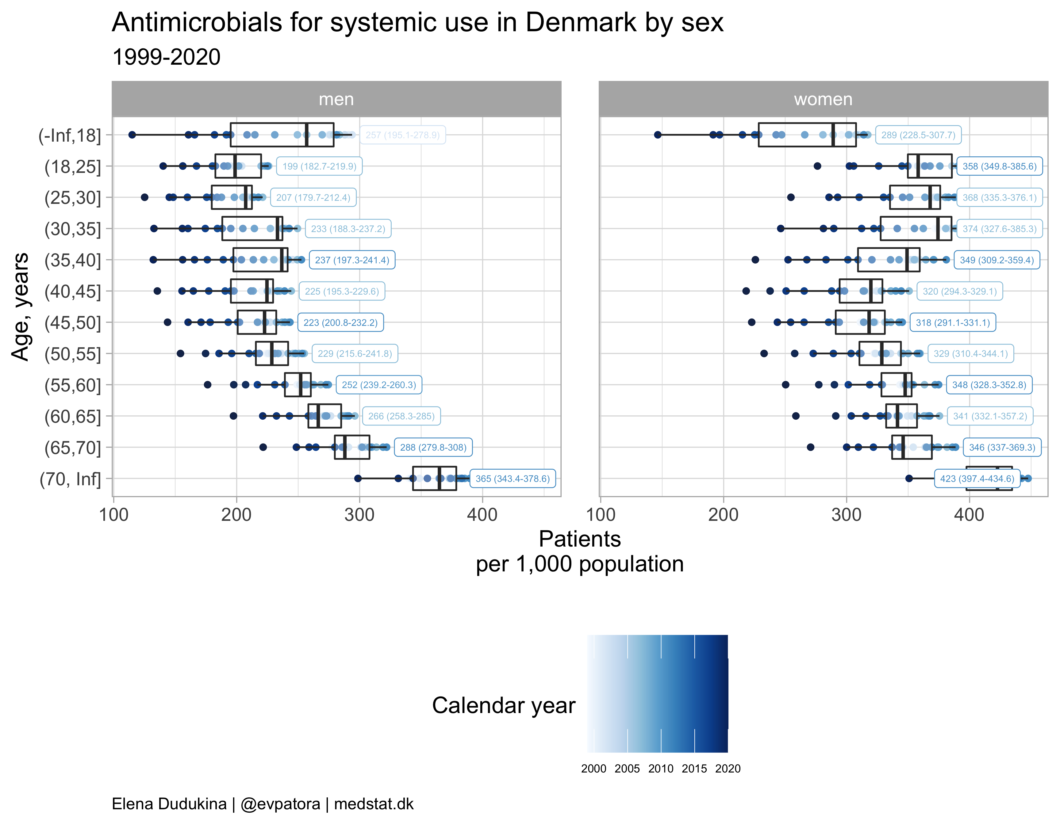
Focus on utilization rate instead of secular trend
atc_data %>%
  filter(str_detect(ATC, regex_AB)) %>%
  mutate(age_cat = fct_rev(age_cat)) %>%
  group_by(age_cat, gender) %>%
  mutate(label = case_when(
   patients_per_1000_inhabitants == max(patients_per_1000_inhabitants) ~ paste0(round(median(patients_per_1000_inhabitants, 1)), " (", round(quantile(patients_per_1000_inhabitants, probs = 0.25), 1), "-",  round(quantile(patients_per_1000_inhabitants, probs = 0.75), 1), ")"),
    T ~ NA_character_
  )) %>%
  ungroup() %>%
  ggplot(aes(x = age_cat, y = patients_per_1000_inhabitants, color = year)) +
  geom_point() +
  geom_boxplot(alpha = 0.3) +
  facet_grid(cols = vars(gender_text)) +
  theme_light(base_size = 14) +
  scale_color_gradientn(colours = RColorBrewer::brewer.pal(name = "Blues", n = 21)) +
  coord_flip() +
  theme(plot.caption = element_text(hjust = 0, size = 10),
        legend.position = "bottom", legend.text = element_text(size = 7),
        panel.spacing = unit(0.8, "cm")) +
  labs(y = "Patients\nper 1,000 population\n", title = "Antimicrobials for systemic use in Denmark by sex", subtitle = "1999-2020", caption = "Elena Dudukina | @evpatora | medstat.dk", x = "Age, years") +
  guides(color = guide_colorbar("Calendar year", barheight = 5))  +
  ggrepel::geom_label_repel(aes(label = label, na.rm = TRUE), direction = "x", segment.size = 0.2, segment.colour = "grey", show.legend = F, size = 2, nudge_y = 1, hjust = 0.5, max.overlaps = 20)
## Warning in RColorBrewer::brewer.pal(name = "Blues", n = 21): n too large, allowed maximum for palette Blues is 9
## Returning the palette you asked for with that many colors

## Warning: Ignoring unknown aesthetics: na.rm

## Warning: Removed 480 rows containing missing values (geom_label_repel).
Output similar plots for each antimicrobial ATC sub-class
plot_use <- function(atc_data, drug_regex, title){
  atc_data %>%
  filter(str_detect(ATC, {{drug_regex}})) %>%
  mutate(label = if_else(year == max(year), as.character(age_cat), NA_character_)) %>%
  ggplot(aes(x = year, y = patients_per_1000_inhabitants, color = age_cat)) +
  geom_path(position = position_dodge(width = 1)) +
  facet_grid(cols = vars(gender_text)) +
  theme_light(base_size = 14) +
  scale_x_continuous(limits = c(1999, 2026), breaks = c(seq(1999, 2020, 10))) +
  scale_y_continuous(position = "right") +
  scale_color_manual(values = wes_palette(name = "GrandBudapest1", type = "continuous", n = 12)) +
  theme(plot.caption = element_text(hjust = 0, size = 10),
        legend.position = "none",
        panel.spacing = unit(0.8, "cm")) +
  labs(y = "Patients\nper 1,000 population\n", title = paste0(title, " use in Denmark by sex"), subtitle = "1999-2020", caption = "Elena Dudukina | @evpatora | medstat.dk") +
  ggrepel::geom_label_repel(aes(label = label, na.rm = TRUE), direction = "y", segment.size = 0.2, segment.colour = "grey", show.legend = F, size = 3.5, nudge_x = 5, hjust = 0.5, max.overlaps = 20)
}

list_regex <- list(regex_TETRACYCLINES, regex_AMPHENICOLS, regex_BETALACTAMS, regex_OTHER_BETALACTAMS, regex_SULFONAMIDES_TRIMETHOPRIM, regex_MACROLIDES_LINCOSAMIDES_STREPTOGRAMINS, regex_AMINOGLYCOSIDES, regex_QUINOLONES)
list_title <- list("Tetracyclines", "Amphenicols", "Beta-lactam antibacterials, penicillins", "Other beta-lactams", "Sulfonamides or trimetoprim", "Macrolides, lincosamides, streptogramins", "Aminoglycosides", "Quinolones")
list_plots <- map2(list_regex, list_title, ~plot_use(atc_data = atc_data, drug_regex = .x, title = .y))
Results
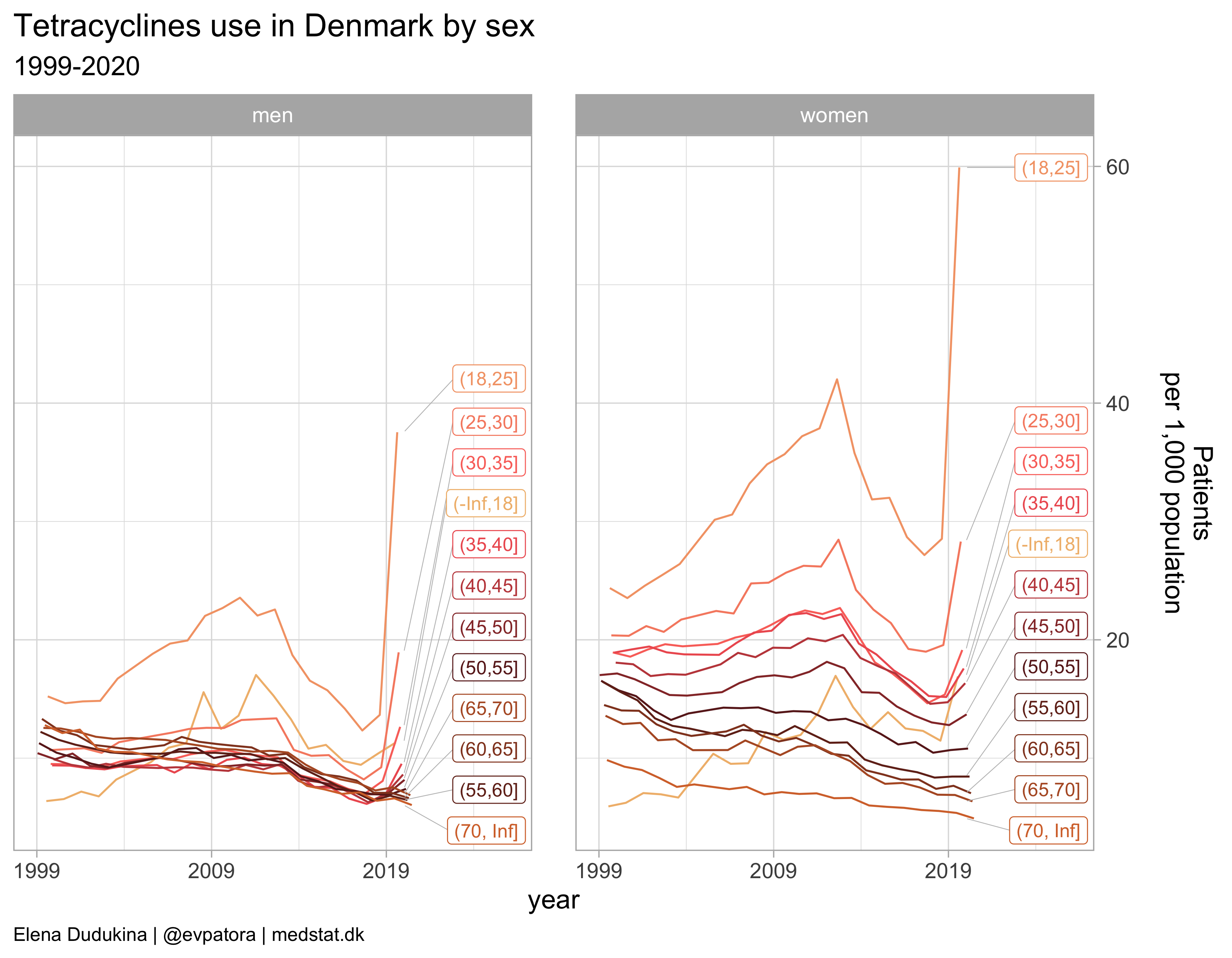
Tetracyclines
list_plots[[1]]
Amphenicols
list_plots[[2]]
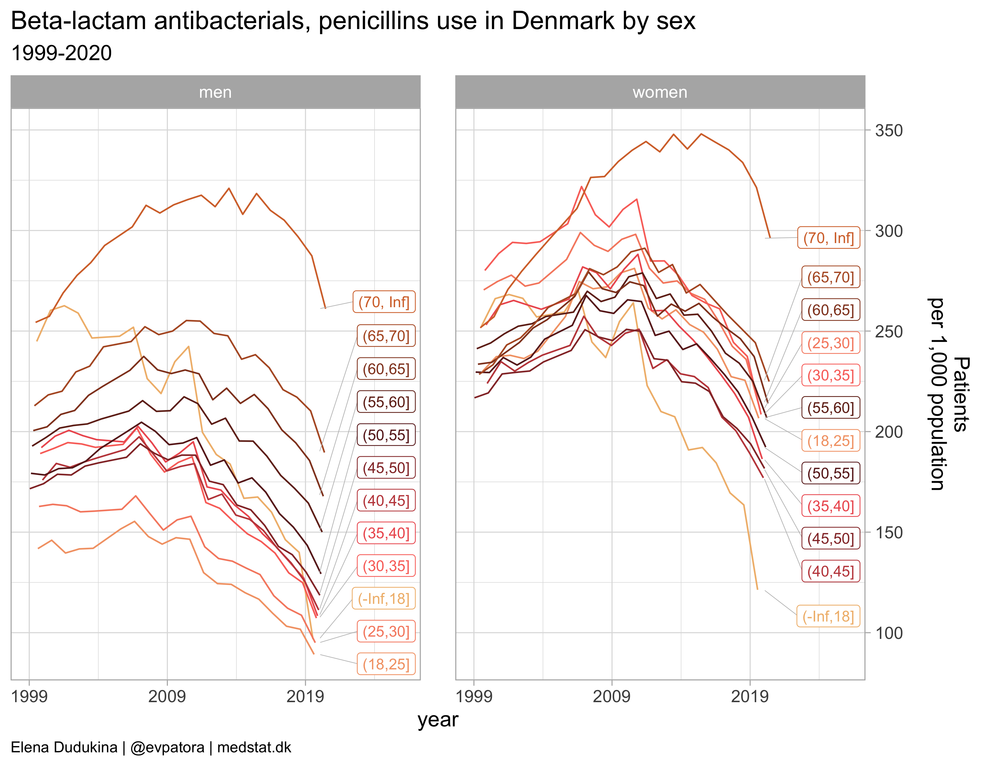
Beta-lactam antibacterials, penicillins
list_plots[[3]]
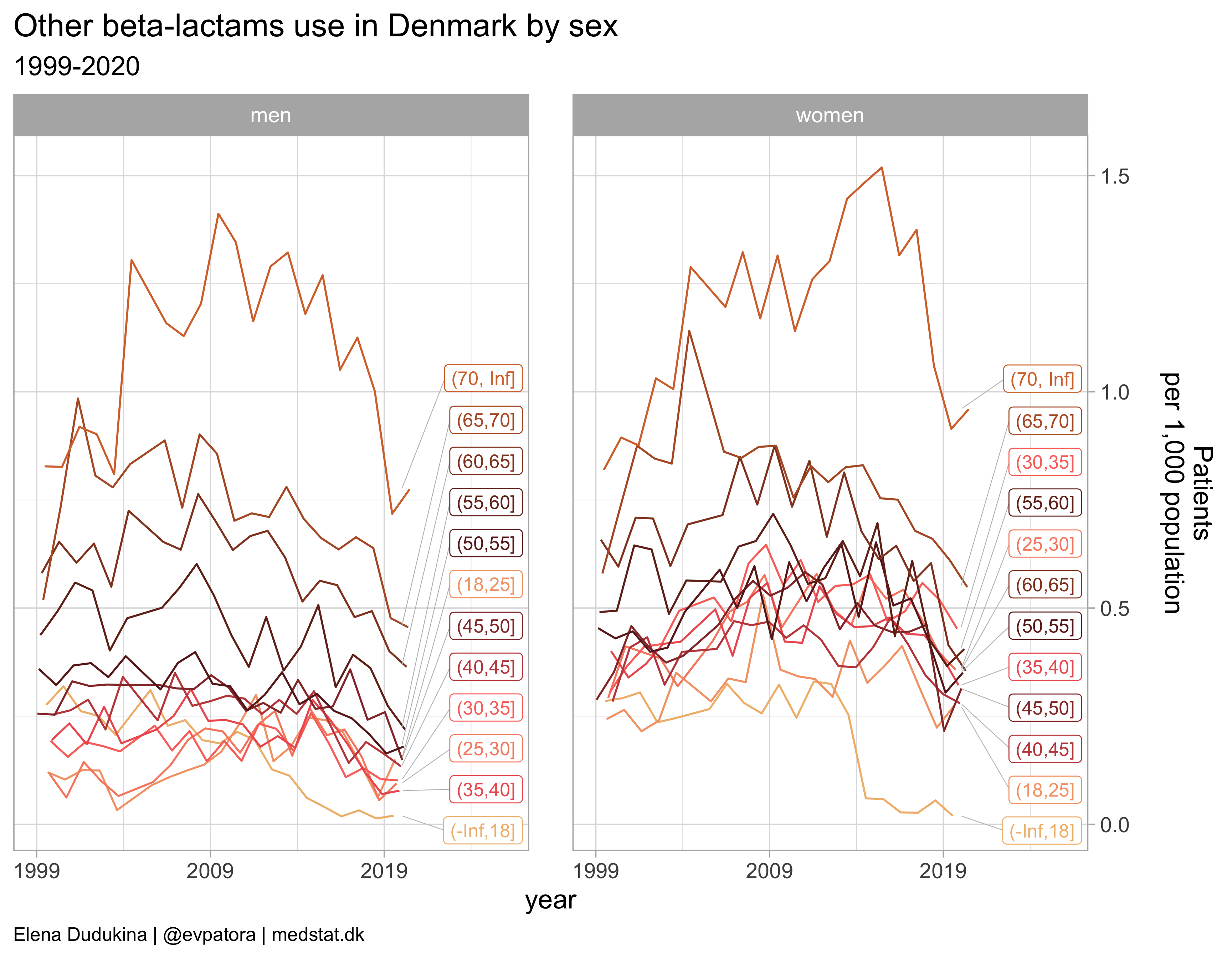
Other beta-lactams
list_plots[[4]]
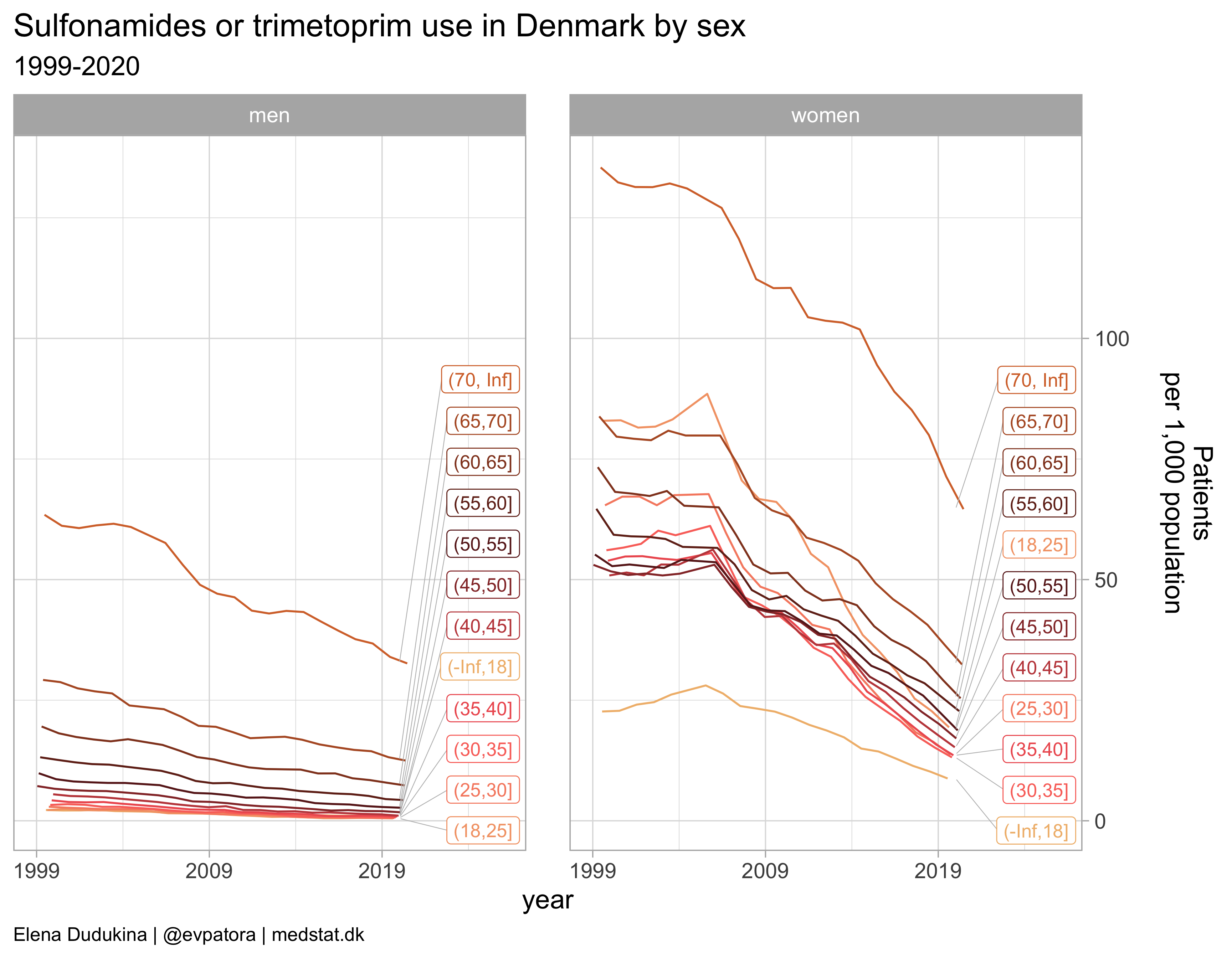
Sulfonamides or trimetoprim
list_plots[[5]]
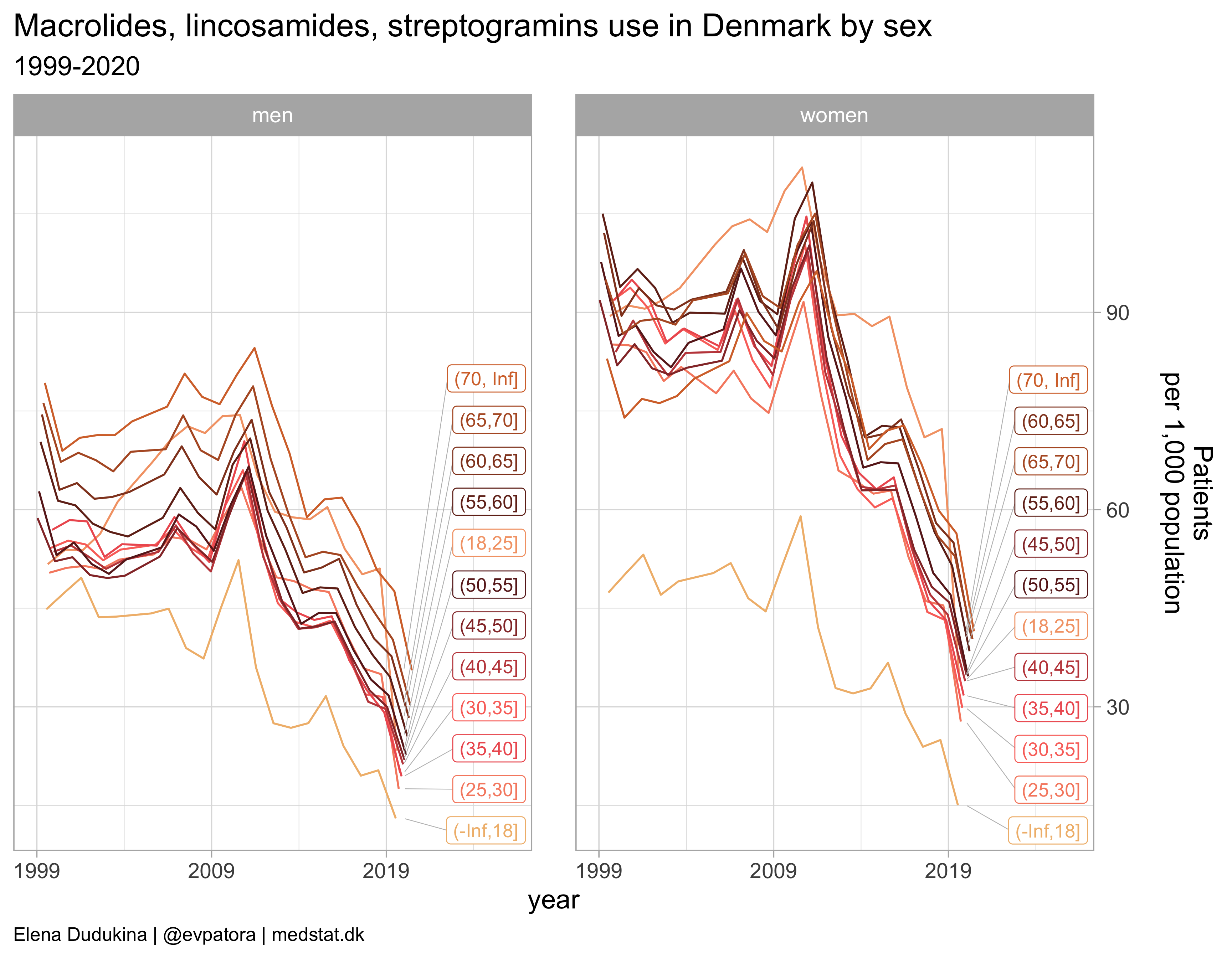
Macrolides, lincosamides, streptogramins
list_plots[[6]]
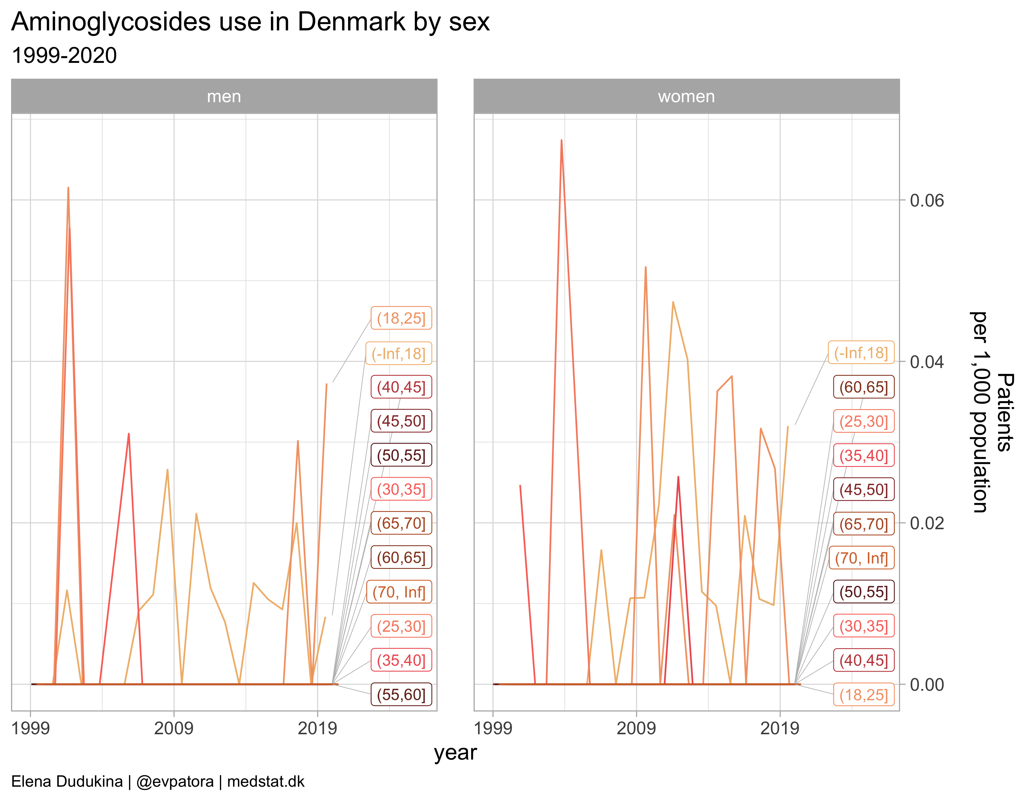
Aminoglycosides
list_plots[[7]]
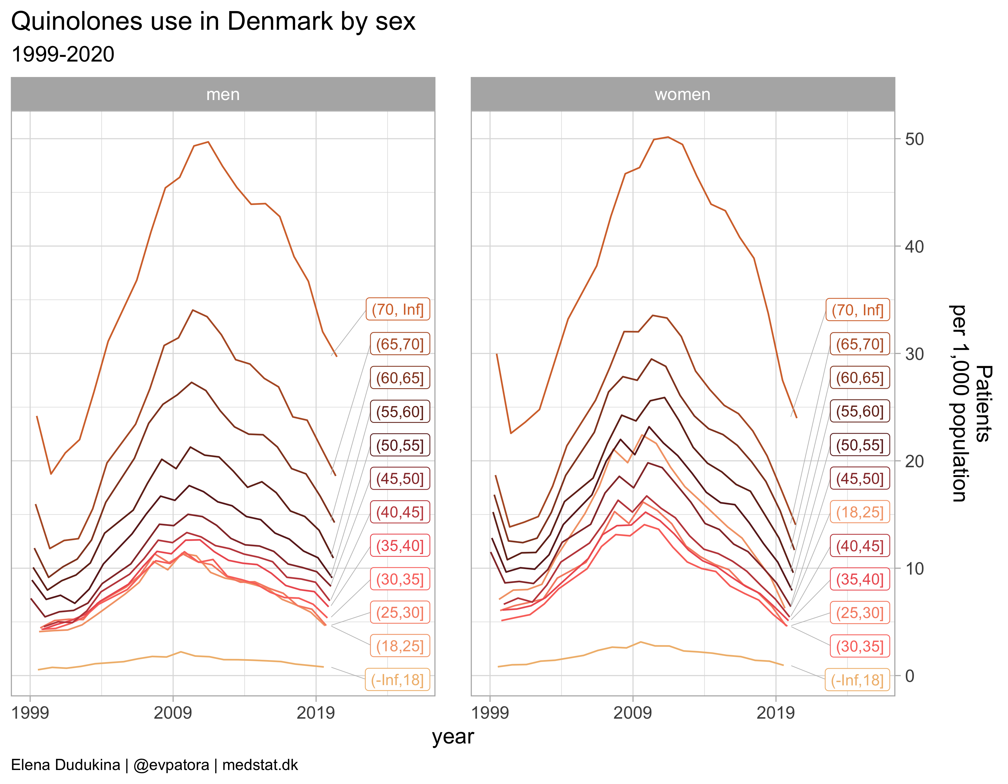
Quinolones
list_plots[[8]]
Final results table for the specific age groups of interest: children and elderly in 2019-2020
atc_data %>%
  filter(age_cat %in% c("(-Inf,18]", "(65,70]", "(70, Inf]"), year %in% c(2019:2020)) %>%
  mutate(patients_per_1000_inhabitants = round(patients_per_1000_inhabitants, 1)) %>%
  select(Gender = gender_text, Age = age_cat, Year = year, ATC, Drug = drug, "Use, per 1000 capita" = patients_per_1000_inhabitants) %>%
  pivot_wider(names_from = c(Age, Gender), values_from = "Use, per 1000 capita", names_sep = ", ") %>%
  arrange(ATC) %>%
  gt::gt(.) %>%
  gt::tab_header(.,
    title = "Antibacterials for systemic use in vulnerable age groups by sex, Denmark, 2019-2020",
    subtitle = "Drug use, per 1000 capita of the underlying population (age group, sex)"
  )
| Antibacterials for systemic use in vulnerable age groups by sex, Denmark, 2019-2020 | ||||||||
|---|---|---|---|---|---|---|---|---|
| Drug use, per 1000 capita of the underlying population (age group, sex) | ||||||||
| Year | ATC | Drug | (-Inf,18], women | (-Inf,18], men | (65,70], women | (65,70], men | (70, Inf], women | (70, Inf], men |
| 2019 | J01 | Antibacterials for systemic use | 191.5 | 160.8 | 300.0 | 248.5 | 385.4 | 331.4 |
| 2020 | J01 | Antibacterials for systemic use | 146.4 | 115.0 | 270.7 | 221.5 | 350.8 | 298.6 |
| 2019 | J01A | Tetracyclines | 11.5 | 10.4 | 6.9 | 7.5 | 5.4 | 6.6 |
| 2020 | J01A | Tetracyclines | 16.9 | 11.3 | 6.4 | 6.9 | 4.9 | 6.0 |
| 2019 | J01C | Beta-lactam antibacterials, penicillins | 163.5 | 139.9 | 244.2 | 210.3 | 321.4 | 287.4 |
| 2020 | J01C | Beta-lactam antibacterials, penicillins | 121.3 | 96.8 | 224.9 | 189.6 | 296.2 | 261.1 |
| 2019 | J01D | Other beta-lactam antibacterials | 0.1 | 0.0 | 0.6 | 0.5 | 0.9 | 0.7 |
| 2020 | J01D | Other beta-lactam antibacterials | 0.0 | 0.0 | 0.5 | 0.5 | 1.0 | 0.8 |
| 2019 | J01E | Sulfonamides and trimethoprim | 10.2 | 0.9 | 36.4 | 13.2 | 71.4 | 34.0 |
| 2020 | J01E | Sulfonamides and trimethoprim | 8.8 | 1.0 | 32.4 | 12.5 | 64.6 | 32.6 |
| 2019 | J01F | Macrolides, lincosamides and streptogramins | 24.9 | 20.3 | 52.9 | 40.2 | 56.4 | 47.6 |
| 2020 | J01F | Macrolides, lincosamides and streptogramins | 15.0 | 13.0 | 40.3 | 30.3 | 41.5 | 35.5 |
| 2019 | J01G | Aminoglycoside antibacterials | 0.0 | 0.0 | 0.0 | 0.0 | 0.0 | 0.0 |
| 2020 | J01G | Aminoglycoside antibacterials | 0.0 | 0.0 | 0.0 | 0.0 | 0.0 | 0.0 |
| 2019 | J01M | Quinolone antibacterials | 1.3 | 0.9 | 17.3 | 21.2 | 27.5 | 32.0 |
| 2020 | J01M | Quinolone antibacterials | 1.0 | 0.8 | 14.0 | 18.6 | 24.0 | 29.7 |
Conclusions
- Antibiotics use varied substantially over time
- Women were prescribed antibiotics at a higher rate than men when looking at J01 ATC code overall; the same pattern held for nearly all J01* subclasses as well
- Among potentially vulnerable age groups (< 18 years, > 66 years), girls and women had higher utilization rates of all antibacterials for systemic use, beta-lactam antibacterials, penicillins, sulfonamides and trimethoprim, macrolides, and lincosamides and streptogramins.
Take home message
tidyverseand expeciallyggplotare useful tools in epidemiology to aggregate, summarize, and visualize data- Both temporal trends and focused descriptive summaries can be compiled in using
tidyverseandgt