Drug utilization in Sweden and Denmark
Part II
In this post (Part II), I will look into the Danish national trends on of sedatives, antidepressants, anti-psychotics and anxiolytics utilization in women. Then I’d like to compare Danish national trends with Swedish national trends from Part I.
library(tidyverse)
library(magrittr)
library(wesanderson)
Dataset
First things first - uploading data.
link_list_dk <- list(
  "1996_atc_code_data.txt" = "https://medstat.dk/da/download/file/MTk5Nl9hdGNfY29kZV9kYXRhLnR4dA==",
  "1997_atc_code_data.txt"  = "https://medstat.dk/da/download/file/MTk5N19hdGNfY29kZV9kYXRhLnR4dA==",
  "1998_atc_code_data.txt" = "https://medstat.dk/da/download/file/MTk5OF9hdGNfY29kZV9kYXRhLnR4dA==",
  "1999_atc_code_data.txt" = "https://medstat.dk/da/download/file/MTk5OV9hdGNfY29kZV9kYXRhLnR4dA==",
  "2000_atc_code_data.txt" = "https://medstat.dk/da/download/file/MjAwMF9hdGNfY29kZV9kYXRhLnR4dA==",
  "2001_atc_code_data.txt" = "https://medstat.dk/da/download/file/MjAwMV9hdGNfY29kZV9kYXRhLnR4dA==",
  "2002_atc_code_data.txt" = "https://medstat.dk/da/download/file/MjAwMl9hdGNfY29kZV9kYXRhLnR4dA==",
  "2003_atc_code_data.txt" = "https://medstat.dk/da/download/file/MjAwM19hdGNfY29kZV9kYXRhLnR4dA==",
  "2004_atc_code_data.txt" = "https://medstat.dk/da/download/file/MjAwNF9hdGNfY29kZV9kYXRhLnR4dA==",
  "2006_atc_code_data.txt" = "https://medstat.dk/da/download/file/MjAwNl9hdGNfY29kZV9kYXRhLnR4dA==",
  "2007_atc_code_data.txt" = "https://medstat.dk/da/download/file/MjAwN19hdGNfY29kZV9kYXRhLnR4dA==",
  "2008_atc_code_data.txt" = "https://medstat.dk/da/download/file/MjAwOF9hdGNfY29kZV9kYXRhLnR4dA==",
  "2009_atc_code_data.txt" = "https://medstat.dk/da/download/file/MjAwOV9hdGNfY29kZV9kYXRhLnR4dA==",
  "2010_atc_code_data.txt" = "https://medstat.dk/da/download/file/MjAxMF9hdGNfY29kZV9kYXRhLnR4dA==",
  "2011_atc_code_data.txt" = "https://medstat.dk/da/download/file/MjAxMV9hdGNfY29kZV9kYXRhLnR4dA==",
  "2012_atc_code_data.txt" = "https://medstat.dk/da/download/file/MjAxMl9hdGNfY29kZV9kYXRhLnR4dA==",
  "2013_atc_code_data.txt" = "https://medstat.dk/da/download/file/MjAxM19hdGNfY29kZV9kYXRhLnR4dA==",
  "2014_atc_code_data.txt" = "https://medstat.dk/da/download/file/MjAxNF9hdGNfY29kZV9kYXRhLnR4dA==",
  "2015_atc_code_data.txt" = "https://medstat.dk/da/download/file/MjAxNV9hdGNfY29kZV9kYXRhLnR4dA==",
  "2016_atc_code_data.txt" = "https://medstat.dk/da/download/file/MjAxNl9hdGNfY29kZV9kYXRhLnR4dA==",
  "2017_atc_code_data.txt" = "https://medstat.dk/da/download/file/MjAxN19hdGNfY29kZV9kYXRhLnR4dA==",
  "2018_atc_code_data.txt" = "https://medstat.dk/da/download/file/MjAxOF9hdGNfY29kZV9kYXRhLnR4dA==",
  "2019_atc_code_data.txt" = "https://medstat.dk/da/download/file/MjAxOV9hdGNfY29kZV9kYXRhLnR4dA==",
  "atc_code_text.txt" = "https://medstat.dk/da/download/file/YXRjX2NvZGVfdGV4dC50eHQ=",
  "atc_groups.txt" = "https://medstat.dk/da/download/file/YXRjX2dyb3Vwcy50eHQ=",
  "population_data.txt" = "https://medstat.dk/da/download/file/cG9wdWxhdGlvbl9kYXRhLnR4dA=="
)

# ATC codes are stored in files
seq_atc <- c(1:23)
atc_code_data_list <- link_list_dk[seq_atc]
I will compile data on population size, which I may use to compute denominators for drug utilization per capita.
# age structure data
# parse with column type character
age_structure <- read_delim(link_list_dk[["population_data.txt"]], delim = ";", col_names = c(paste0("V", c(1:7))), col_types = cols(V1 = col_character(), V2 = col_character(), V3 = col_character(), V4 = col_character(), V5 = col_character(), V6 = col_character(), V7 = col_character())) %>%
  # rename and keep columns
  select(year = V1,
         region_text = V2,
         region = V3,
         gender = V4,
         age = V5,
         denominator_per_year = V6) %>%
  # human-reading friendly label on sex categories
  mutate(
      gender_text = case_when(
      gender == "0" ~ "both sexes",
      gender == "1" ~ "men",
      gender == "2" ~ "women",
      T ~ as.character(gender)
    )
  ) %>%
  # make numeric variables
  mutate_at(vars(year, age, denominator_per_year), as.numeric) %>%
  # keep only data for the age categories I will work with and only on women
  filter(age %in% 20:54, gender == "2") %>%
  arrange(year, age, region, gender)

age_structure %>% slice(1:10)
## # A tibble: 10 x 7
##     year region_text region gender   age denominator_per_year gender_text
##    <dbl> <chr>       <chr>  <chr>  <dbl>                <dbl> <chr>
##  1  1996 DK          0      2         20                36363 women
##  2  1996 DK          0      2         21                36366 women
##  3  1996 DK          0      2         22                36498 women
##  4  1996 DK          0      2         23                38452 women
##  5  1996 DK          0      2         24                37873 women
##  6  1996 DK          0      2         25                36383 women
##  7  1996 DK          0      2         26                36115 women
##  8  1996 DK          0      2         27                37514 women
##  9  1996 DK          0      2         28                40669 women
## 10  1996 DK          0      2         29                43619 women
Danish data has a handy file with all drug classes in English, which I intend to use as labels later on.
eng_drug <- read_delim(link_list_dk[["atc_groups.txt"]], delim = ";", col_names = c(paste0("V", c(1:6))), col_types = cols(V1 = col_character(), V2 = col_character(), V3 = col_character(), V4 = col_character(), V5 = col_character(), V6 = col_character())) %>%
  # keep drug classes labels in English
  filter(V5 == "1") %>%
  select(ATC = V1,
         drug = V2,
         unit_dk = V4)

eng_drug %>% slice(1:10)
## # A tibble: 10 x 3
##    ATC     drug                                    unit_dk
##    <chr>   <chr>                                   <chr>
##  1 A       Alimentary tract and metabolism         No common unit for volume
##  2 A01     Stomatological preparations             No common unit for volume
##  3 A01A    Stomatological preparations             No common unit for volume
##  4 A01AA   Caries prophylactic agents              Packages
##  5 A01AA01 Sodium fluoride                         Packages
##  6 A01AB   Antiinfectives for local oral treatment No common unit for volume
##  7 A01AB02 Hydrogenperoxide                        <NA>
##  8 A01AB03 Chlorhexidine                           DDD
##  9 A01AB04 Amphotericin                            DDD
## 10 A01AB09 Miconazole                              DDD
I keep only ATC codes I am interested in. I use $ in the end of each regular expression (regex) to make sure that I capture the widest ATC code category, which already encompasses all the subcategories. Hypnotics and sedatives - N05C already aggregates N05CA, N05CB, N05CC, N05CD, N05CE, N05CF, N05CH ATC codes.
regex_antidepress <- "^N06A$"
regex_antipsych <- "^N05A$"
regex_anxiolyt <- "^N05B$"
regex_sedat <- "^N05C$"

# combine all ATC codes in one regex string
all_regex <- paste(regex_antidepress, regex_antipsych, regex_anxiolyt, regex_sedat, sep = "|")
# ATC data
atc_data <- map(atc_code_data_list, ~read_delim(file = .x, delim = ";", trim_ws = T, col_names = c(paste0("V", c(1:14))), col_types = cols(V1 = col_character(), V2 = col_character(), V3 = col_character(), V4 = col_character(), V5 = col_character(),V6 = col_character(), V7 = col_character(), V8 = col_character(), V9 = col_character(), V10 = col_character(), V11 = col_character(), V12 = col_character(), V13 = col_character(), V14 = col_character()))) %>%
  # bind data from all years
  bind_rows()

# age categories: in 6 year bands and in each year
age_cat_in_6 <- atc_data %>% distinct(V6) %>% filter(row_number() %in% 2:7) %>% pull()
age_cat_in_6
## [1] "00-17" "18-24" "25-44" "45-64" "65-79" "80+"
age_in_years <- atc_data %>% distinct(V6) %>% filter(row_number() %in% 8:103) %>% pull()
age_in_years
##  [1] "000" "001" "002" "003" "004" "005" "006" "007" "008" "009" "010" "011"
## [13] "012" "013" "014" "015" "016" "017" "018" "019" "020" "021" "022" "023"
## [25] "024" "025" "026" "027" "028" "029" "030" "031" "032" "033" "034" "035"
## [37] "036" "037" "038" "039" "040" "041" "042" "043" "044" "045" "046" "047"
## [49] "048" "049" "050" "051" "052" "053" "054" "055" "056" "057" "058" "059"
## [61] "060" "061" "062" "063" "064" "065" "066" "067" "068" "069" "070" "071"
## [73] "072" "073" "074" "075" "076" "077" "078" "079" "080" "081" "082" "083"
## [85] "084" "085" "086" "087" "088" "089" "090" "091" "092" "093" "094" "95+"
# clean dataset
atc_data %<>%
  # rename and keep columns
  rename(
    ATC = V1,
    year = V2,
    sector = V3,
    region = V4,
    gender = V5, # 0 - both; 1 - male; 2 - female
    age = V6,
    number_of_people = V7,
    patients_per_1000_inhabitants = V8,
    turnover = V9,
    regional_grant_paid = V10,
    quantity_sold_1000_units = V11,
    quantity_sold_units_per_unit_1000_inhabitants_per_day = V12,
    percentage_of_sales_in_the_primary_sector = V13
  ) %>%
  # clean columns names and set-up labels
  mutate(
    year = as.numeric(year),
    region_text = case_when(
      region == "0" ~ "DK",
      region == "1" ~ "Region Hovedstaden",
      region == "2" ~ "Region Midtjylland",
      region == "3" ~ "Region Nordjylland",
      region == "4" ~ "Region Sjælland",
      region == "5" ~ "Region Syddanmark",
      T ~ NA_character_
    ),
    gender_text = case_when(
      gender == "0" ~ "both sexes",
      gender == "1" ~ "men",
      gender == "2" ~ "women",
      T ~ as.character(gender)
    ),
    age_cats = case_when(
      age %in% "A" ~ "A",
      age %in% age_cat_in_6 ~ "6 years",
      age %in% age_in_years ~ "yearly categories",
      age %in% "T" ~ "T",
      T ~ NA_character_
    )
  ) %>%
  mutate_at(vars(turnover, regional_grant_paid, quantity_sold_1000_units, quantity_sold_units_per_unit_1000_inhabitants_per_day, number_of_people, patients_per_1000_inhabitants), as.numeric) %>%
  select(-V14) %>%
  filter(
  age_cats == "yearly categories",
  gender == "2",
  region == "0",
  sector =="0"
) %>%
  filter(str_detect(ATC, all_regex)) %>%
  # deal with non-numeric age and re-code as numeric
  mutate(
    age = case_when(
      age == "95+" ~ "95",
      T ~ as.character(age)
    ),
    age = as.numeric(age)
    ) %>%
  filter(age %in% 20:54) %>%
  mutate(
    age_cat = case_when(
      age %in% 20:24 ~ "20-24",
      age %in% 25:34 ~ "25-34",
      age %in% 35:44 ~ "35-44",
      age %in% 45:54 ~ "45-54",
      T ~ NA_character_
    )
) %>%
  left_join(age_structure) %>%
  group_by(ATC, year, age_cat) %>%
  mutate(
    numerator = sum(number_of_people),
    denominator = sum(denominator_per_year),
    patients_per_1000_inhabitants = numerator / denominator * 1000
  ) %>%
  filter(row_number() == 1) %>%
  ungroup() %>%
  select(year, ATC, gender, age_cat, patients_per_1000_inhabitants) %>%
  mutate(
    country = "Denmark"
  )
## Joining, by = c("year", "region", "gender", "age", "region_text", "gender_text")
atc_data %>% slice(1:10)
## # A tibble: 10 x 6
##     year ATC   gender age_cat patients_per_1000_inhabitants country
##    <dbl> <chr> <chr>  <chr>                           <dbl> <chr>
##  1  1999 N05A  2      20-24                            5.60 Denmark
##  2  1999 N05A  2      25-34                            9.71 Denmark
##  3  1999 N05A  2      35-44                           19.9  Denmark
##  4  1999 N05A  2      45-54                           29.4  Denmark
##  5  1999 N05B  2      20-24                           12.5  Denmark
##  6  1999 N05B  2      25-34                           26.3  Denmark
##  7  1999 N05B  2      35-44                           61.7  Denmark
##  8  1999 N05B  2      45-54                          106.   Denmark
##  9  1999 N05C  2      20-24                            7.86 Denmark
## 10  1999 N05C  2      25-34                           18.0  Denmark
Combining Danish and Swedish data
# combine Swedish data from previous post and Danish data
data <- data_se %>%
  select(year, ATC, gender, age_cat, patients_per_1000_inhabitants) %>%
  mutate(
    country = "Sweden"
  ) %>%
  full_join(atc_data) %>%
  # join with ATC classes labels in English
  left_join(eng_drug)
## Joining, by = c("year", "ATC", "gender", "age_cat", "patients_per_1000_inhabitants", "country")
## Joining, by = "ATC"
To avoid copy-pasting the same ggplot code, I use a wrapper around the plotting function.
plot_utilization <- function(data, drug_regex, title){
  data %>%
  filter(str_detect(ATC, {{ drug_regex }})) %>%
  group_by(country) %>%
  ggplot(aes(x = year, y = patients_per_1000_inhabitants, color = country)) +
  geom_path(position = position_dodge(width = 1)) +
  facet_grid(rows = vars(drug, ATC), cols = vars(age_cat), scales = "free", drop = T) +
  theme_light(base_size = 14) +
  scale_x_continuous(breaks = c(seq(1999, 2019, 10))) +
  scale_color_manual(values = wes_palette(name = "GrandBudapest1", type = "discrete")) +
  theme(plot.caption = element_text(hjust = 0, size = 10),
        legend.position = "bottom",
        panel.spacing = unit(0.8, "cm")) +
  labs(y = "Female patients\nper 1,000 women in the population", title = paste0(title, " utilization in Swedish and Danish women"), subtitle = "aged between 20 and 54 years", caption = "dataviz by Elena Dudukina Twitter @evpatora\nSources: sdb.socialstyrelsen.se; medstat.dk")
}

list_regex <- list(regex_antidepress, regex_antipsych, regex_anxiolyt, regex_sedat)
list_title <- list("Antidepressants", "Antipsychotics", "Anxiolytics", "Sedatives")
list_plots <- map2(list_regex, list_title, ~plot_utilization(data = data, drug_regex = .x, title = .y))
Results
list_plots[[1]]
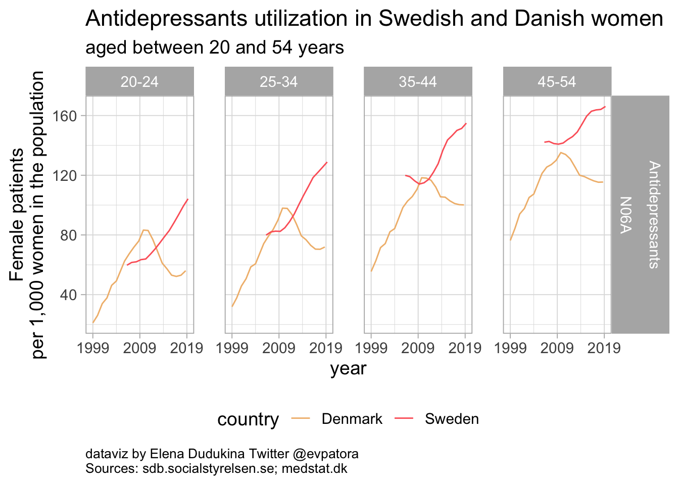 ### Antidepressants
Among Danish women aged between 20 and 54 years, antidepressants utilizatioin was steadily decreasing, while utilization among Swedish women was increasing. In Denmark, 56 women aged between 20-24 and 72 women aged between 35-45 per 1000 women in the population received antidepressants prescription.
### Antidepressants
Among Danish women aged between 20 and 54 years, antidepressants utilizatioin was steadily decreasing, while utilization among Swedish women was increasing. In Denmark, 56 women aged between 20-24 and 72 women aged between 35-45 per 1000 women in the population received antidepressants prescription.
list_plots[[2]]
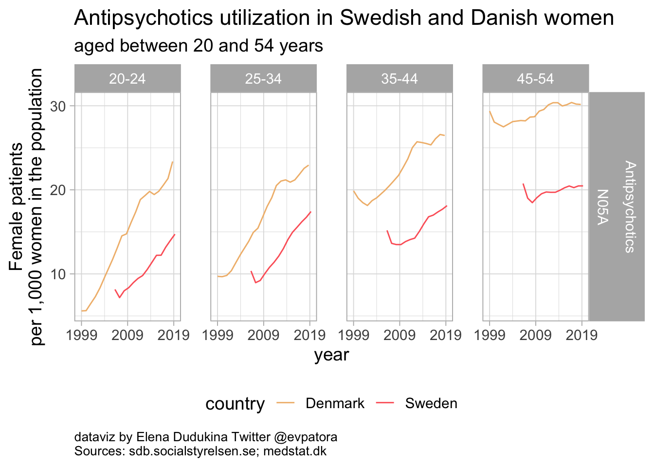
Antipsychotics
Antipsychotics utilization was increasing over the years in both Denmark and Sweden. The rates of antipsychotics utilization were higher among Danish women when compared to Swedish women in the same age categories.
list_plots[[3]]
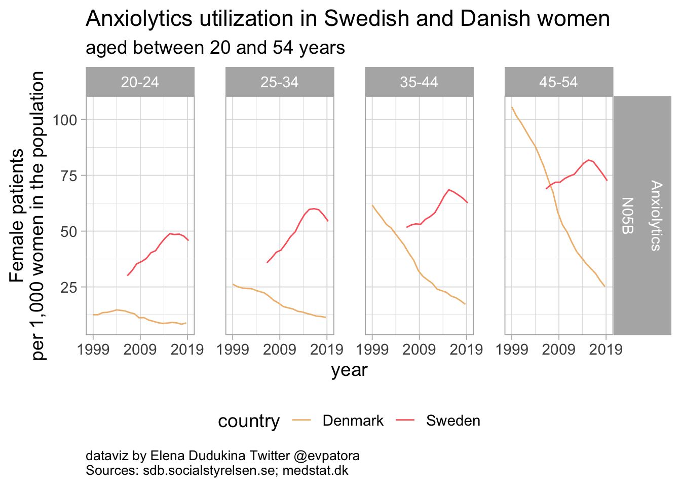
Anxiolytics
Anxiolytics utilization rates were higher among Swedish women. In Denmark, anxiolytics utilization was decreasing since 1999 until 2019 for women in all age categories between 20 and 54 years.
list_plots[[4]]
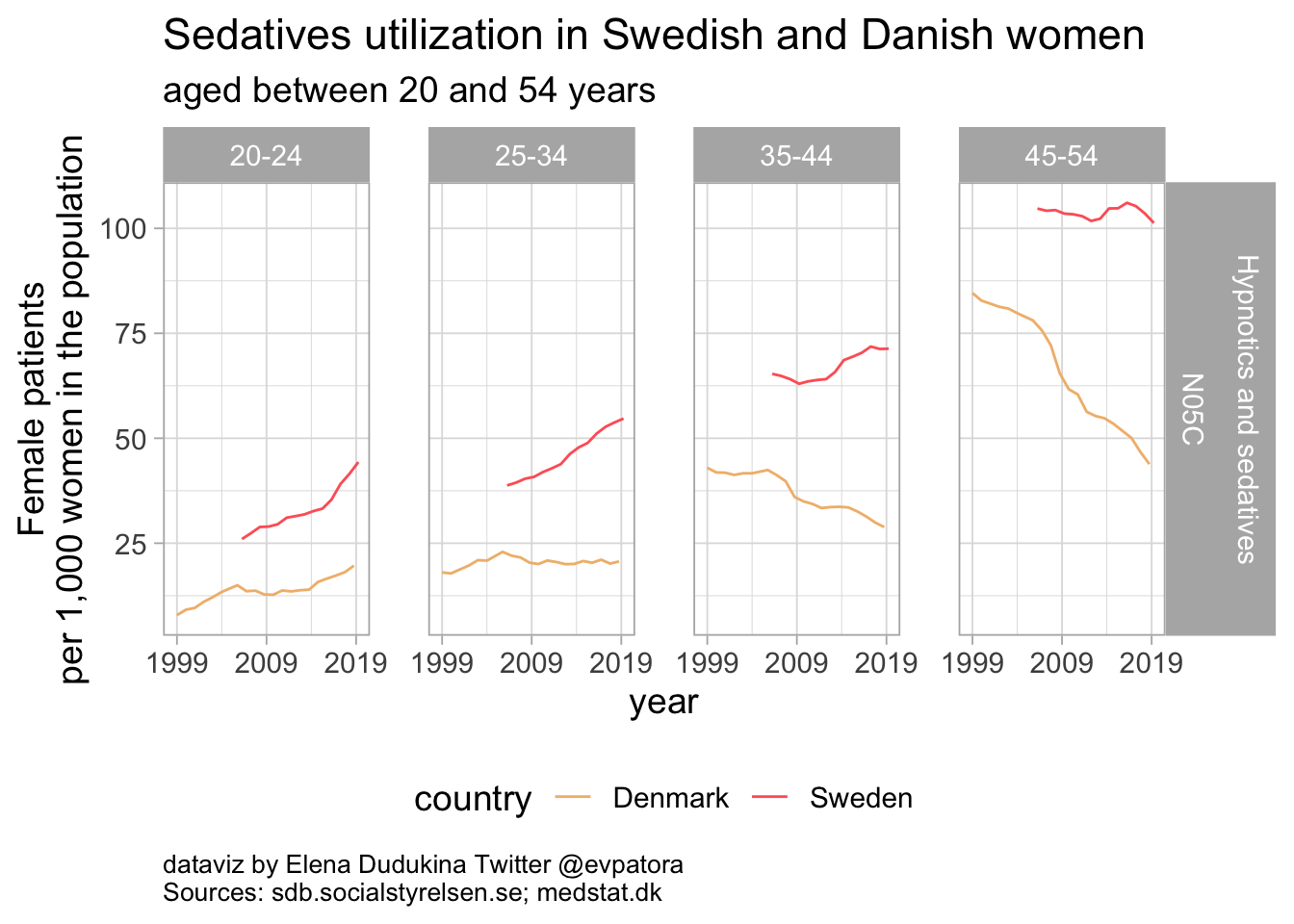
Sedatives
The rates of sedatives utilization were higher for Swedish women when compared with Danish women of the same age groups. Utilization of sedatives among Danish women was below 50 women per 1000 women of the same age group in the population in all investigated age categories. Among Swedish women, the rate of sedatives utilization was below 50 women per 1000 women in the population only for women between 20 and 24 years of age.
Take home message
- Countries similar in many ways may exhibit different data patterns
- Antidepressants, antipsychotics, anxiolytics, and sedatives utilization among Danish and Swedish women is far from identical
Thanks for tuning in 🤓
All feedback is appreciated ✌️