Iterative visualizations with ggplot2: no more copy-pasting
Are you tired of copy-pasting some chunks of your code over and over again? I am, too. Let’s dig into how we can improve our workflow with a bit of tidy evaluation and writing our own functions to avoid copy-pasting.
Download the dataset here
Tidy (non-standard) evaluation
- Data masking
- How code is being quoted
- How code is being unquoted
Lots of materials on the topic of tidy evaluation here: https://adv-r.hadley.nz/
# data masking: access columns indirectly
# regular (standard) evaluation
data[data$ATC == "N06A" & data$gender_text == "women" & data$year == 1999, ][1:10, ]
## # A tibble: 10 × 20
##    ATC    year sector region gender   age number_of_people patients_per_1000_in…
##    <chr> <dbl> <chr>  <chr>  <chr>  <dbl>            <dbl>                 <dbl>
##  1 N06A   1999 0      0      2          0                0                 0.120
##  2 N06A   1999 0      0      2         11               25                 7.05
##  3 N06A   1999 0      0      2         21              638                25.7
##  4 N06A   1999 0      0      2         31             1357                44.7
##  5 N06A   1999 0      0      2         41             2159                70.1
##  6 N06A   1999 0      0      2         51             3070                83.8
##  7 N06A   1999 0      0      2         61             2556               101.
##  8 N06A   1999 0      0      2         71             2543               136.
##  9 N06A   1999 0      0      2         81             2565               183.
## 10 N06A   1999 0      0      2         91              817               210.
## # … with 12 more variables: turnover <dbl>, regional_grant_paid <dbl>,
## #   quantity_sold_1000_units <dbl>,
## #   quantity_sold_units_per_unit_1000_inhabitants_per_day <dbl>,
## #   percentage_of_sales_in_the_primary_sector <chr>, region_text <chr>,
## #   gender_text <chr>, age_cats <chr>, age_cat <fct>,
## #   denominator_per_year <dbl>, numerator <dbl>, denominator <dbl>
# tidy: with masking .data[[var]] --> var
data %>%
  filter(ATC == "N06A", gender_text == "women", year == 1999) %>%
  slice(1:10)
## # A tibble: 10 × 20
##    ATC    year sector region gender   age number_of_people patients_per_1000_in…
##    <chr> <dbl> <chr>  <chr>  <chr>  <dbl>            <dbl>                 <dbl>
##  1 N06A   1999 0      0      2          0                0                 0.120
##  2 N06A   1999 0      0      2         11               25                 7.05
##  3 N06A   1999 0      0      2         21              638                25.7
##  4 N06A   1999 0      0      2         31             1357                44.7
##  5 N06A   1999 0      0      2         41             2159                70.1
##  6 N06A   1999 0      0      2         51             3070                83.8
##  7 N06A   1999 0      0      2         61             2556               101.
##  8 N06A   1999 0      0      2         71             2543               136.
##  9 N06A   1999 0      0      2         81             2565               183.
## 10 N06A   1999 0      0      2         91              817               210.
## # … with 12 more variables: turnover <dbl>, regional_grant_paid <dbl>,
## #   quantity_sold_1000_units <dbl>,
## #   quantity_sold_units_per_unit_1000_inhabitants_per_day <dbl>,
## #   percentage_of_sales_in_the_primary_sector <chr>, region_text <chr>,
## #   gender_text <chr>, age_cats <chr>, age_cat <fct>,
## #   denominator_per_year <dbl>, numerator <dbl>, denominator <dbl>
# coding means processing the expressions
# quoting: delaying the code execution behind the scenes
# expr() turns things into symbols
# sym() turns strings into symbols

x <- c(2, 2, 4, 4)
mean(x, na.rm = TRUE)
## [1] 3
expr(mean(x, na.rm = TRUE))
## mean(x, na.rm = TRUE)
expr(x)
## x
sym("x")
## x
# many things: exprs() is useful interactively to make a list of expressions
rlang::exprs(x = x * 15, y = d / 3, z = f ^ 2)
## $x
## x * 15
##
## $y
## d/3
##
## $z
## f^2
# shorthand for
# list(x = expr(x * 15), y = expr(d / 3), z = expr(f ^ 2))

# base version of expr() is quote()
quote(1+2)
## 1 + 2
# unquoting: used when it's time to process the quoted expression
# the unquote operator !! (pronounced bang-bang)

xx <- expr(x + x)
yy <- expr(y + y)

expr(xx / yy)
## xx/yy
expr(!!xx / !!yy)
## (x + x)/(y + y)
# !!!, called “unquote-splice”, unquote many arguments
manyexpr <- rlang::exprs(1, a + 3, -b/10)

manyexpr[[1]]
## [1] 1
manyexpr[[2]]
## a + 3
manyexpr[[3]]
## -b/10
expr(f(!!! manyexpr))
## f(1, a + 3, -b/10)
expr(f(!!manyexpr[[1]]) + yy)
## f(1) + yy
Visualization
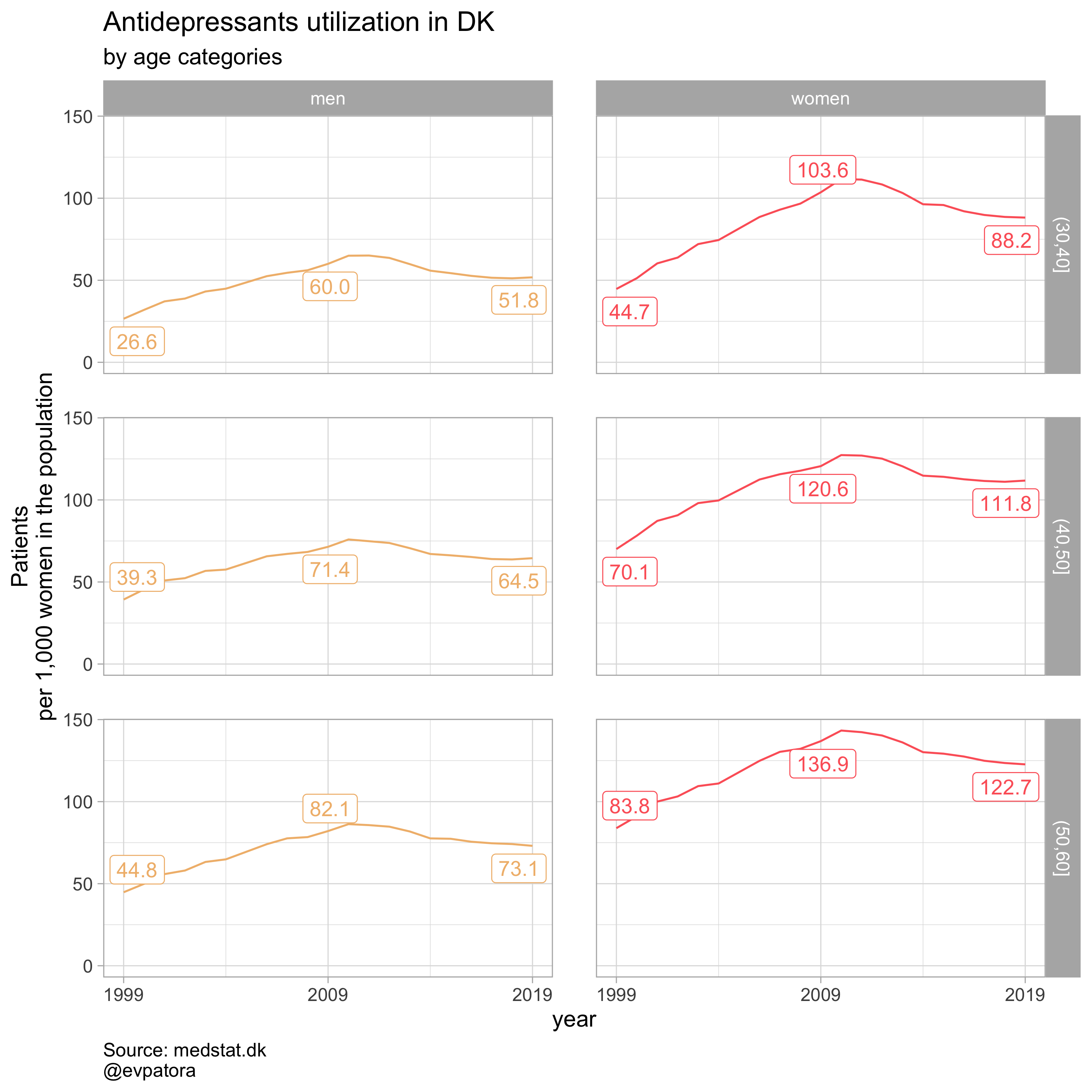
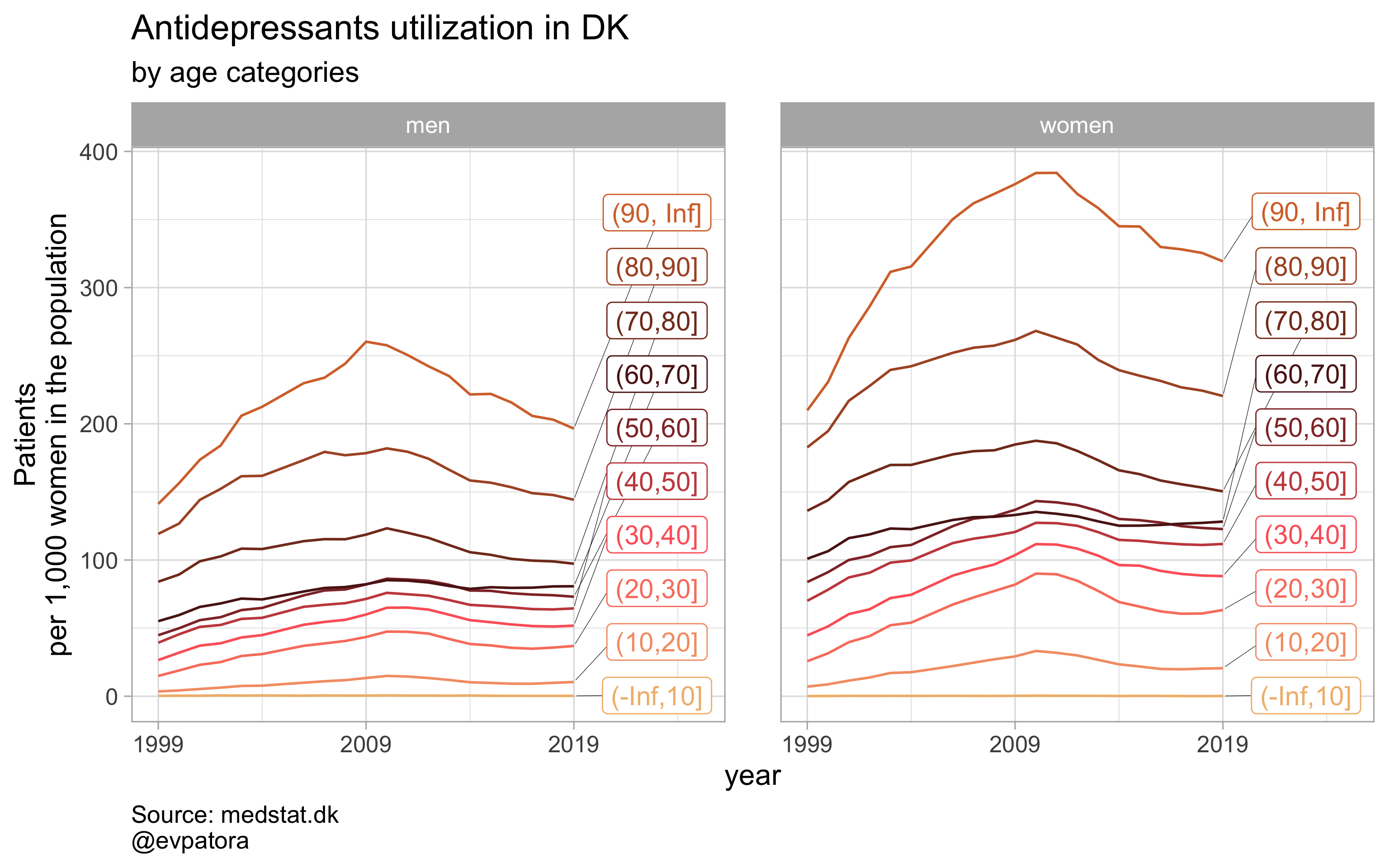
# make a plot of Antidepressants (ATC:N06A) utilization rates in men & women separately 30-50 in 1999-2019, DK

data %>%
  filter(region == "0", str_detect(ATC, "^N06A$"), age_cat %in% c("(30,40]", "(40,50]", "(50,60]")) %>%
  mutate(
      label = if_else(year == 1999 | year == 2009 | year == 2019, as.character(sprintf("%1.1f", round(patients_per_1000_inhabitants, digits = 1))), NA_character_)
    ) %>%
  ggplot(aes(x = year, y = patients_per_1000_inhabitants, color = gender)) +
  geom_path() +
  facet_grid(cols = vars(gender_text), rows = vars(age_cat), scales = "fixed", drop = T) +
  theme_light(base_size = 12) +
  # start y scale at 0
  expand_limits(y = 0) +
  scale_x_continuous(breaks = c(seq(1999, 2019, 10))) +
  ggrepel::geom_label_repel(aes(label = label), na.rm = TRUE, nudge_x = 0.1, direction = "y", segment.size = 0.1, segment.colour = "black", show.legend = F) +
  scale_color_manual(values = wes_palette(name = "GrandBudapest1", type = "discrete")) +
  theme(plot.caption = element_text(hjust = 0, size = 10),
        legend.position = "none",
        panel.spacing = unit(0.8, "cm")) +
  labs(y = "Patients\nper 1,000 women in the population", title = paste0("Antidepressants utilization in DK"), subtitle = "by age categories", caption = "Source: medstat.dk\n@evpatora")
 List of the drugs of interest
regex_antidepress <- "^N06A$"
regex_antipsych <- "^N05A$"
regex_anxiolyt <- "^N05B$"
regex_sedat <- "^N05C$"
Writing ggplot2 wrapper function
In tidyverse instead of quoting and unquoting in 2 separate steps, it can be combined in 1 step with {{ “curly-curly” operator. I take the plotting function above and wrap it inside my custom function. ATC column becomes {{ atc }}, a “curly-curly” operator embraced column, which I as a user will specify when using my custom function. Same logic is applied to data column age_cat, which becomes {{ age_var }}; year column, which becomes {{ year_var }}, etc. Once I worked with all the columns I need to use to produce the wanted graphics and minding that this function may be useful for the same or similar datasets with the columns named differently, I test my custom function.
plot_utilization <- function(.my_data, drug_regex, atc, age_var, year_var, rate_var, sex_var, title){
.my_data %>% # use data pronoun to make the function pipe-able
# filter non-missing values on utilization rates
filter(! is.na({{ rate_var }})) %>%
# filter needed ATC code and age age categories "(30,40]", "(40,50]", "(50,60]"
filter(str_detect({{ atc }}, drug_regex), {{ age_var }} %in% c("(30,40]", "(40,50]", "(50,60]")) %>%
mutate(
label = if_else({{ year_var }} == 1999 | {{ year_var }} == 2009 | {{ year_var }} == 2019, as.character(sprintf("%1.1f", round({{ rate_var }}, digits = 1))), NA_character_)
) %>%
ggplot(aes(x = {{ year_var }}, y = {{ rate_var }}, color = {{ sex_var }})) +
geom_path() +
facet_grid(cols = vars({{ sex_var }}), rows = vars({{ age_var }}), scales = "fixed", drop = T) +
theme_light(base_size = 12) +
scale_x_continuous(breaks = c(seq(1999, 2019, 10))) +
expand_limits(y = 0) +
ggrepel::geom_label_repel(aes(label = label), na.rm = TRUE, nudge_x = 0.1, direction = "y", segment.size = 0.1, segment.colour = "black", show.legend = F) +
theme(plot.caption = element_text(hjust = 0, size = 10),
legend.position = "none",
panel.spacing = unit(0.8, "cm")) +
scale_color_manual(values = wes_palette(name = "GrandBudapest1", type = "discrete")) +
labs(y = "Patients\nper 1,000 women in the population", title = paste0(title, " utilization in DK"), subtitle = "by age categories", caption = "Source: medstat.dk\n@evpatora")
}
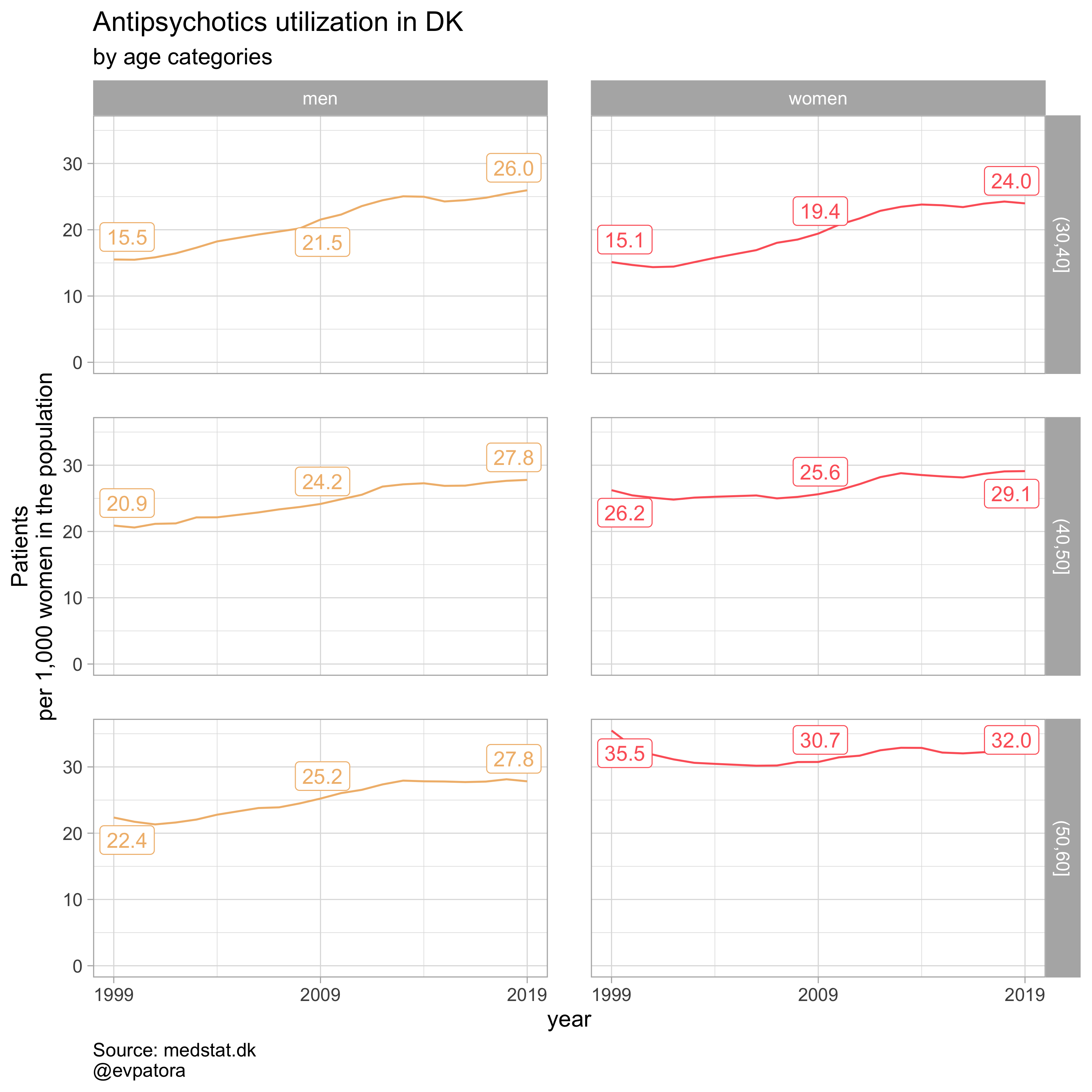
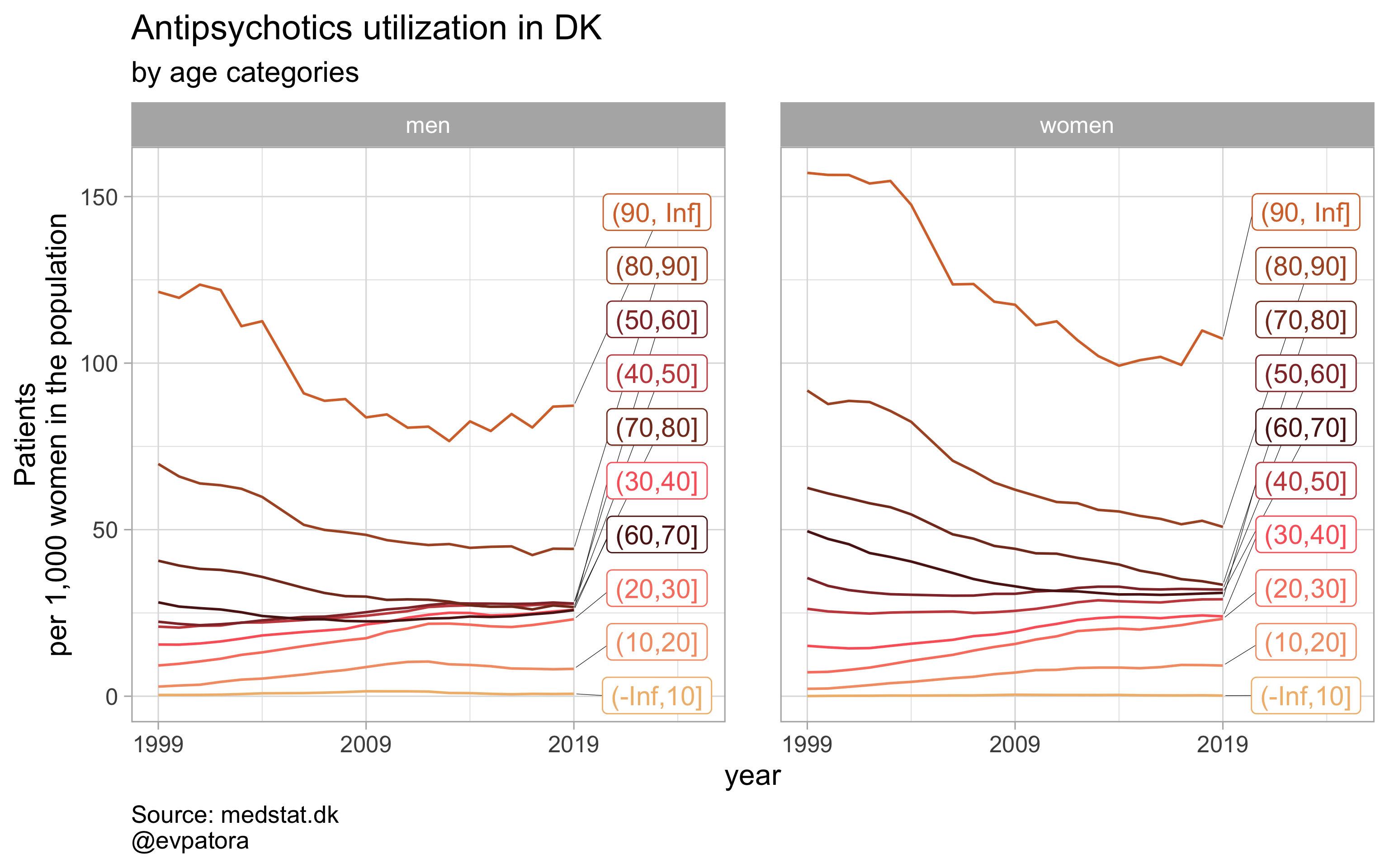
# testing the custom function
data %>%
# I only want the country-level graph, hence `region == 0`
filter(region == "0") %>%
# . is my data pronoun
plot_utilization(., atc = ATC, drug_regex = regex_antipsych, age_var = age_cat, year_var = year, rate_var = patients_per_1000_inhabitants, sex_var = gender_text, title = "Antipsychotics")
 ## Customizing `ggplot2` wrapper function
Adding filtering
Say, I am now only interested in learning the drug utilization rates on the country-level, therefore I want to skip filtering data every time before I run my custom function. I can incorporate this step directly into my custom function.
plot_utilization_region <- function(.my_data, drug_regex, atc, age_var, year_var, rate_var, sex_var, title, region_var = region){
.my_data %>%
# filter non-missing values on utilization rates
filter(! is.na({{ rate_var }})) %>%
# add filtering the region into my custom function minding that the column can be named differently by me or other users of this function, hence region column becomes `{{ region_var }}`
filter({{ region_var }} == "0", str_detect({{ atc }}, drug_regex), {{ age_var }} %in% c("(30,40]", "(40,50]", "(50,60]")) %>%
mutate(
label = if_else({{ year_var }} == 1999 | {{ year_var }} == 2009 | {{ year_var }} == 2019, as.character(sprintf("%1.1f", round({{ rate_var }}, digits = 1))), NA_character_)
) %>%
ggplot(aes(x = {{ year_var }}, y = {{ rate_var }}, color = {{ sex_var }})) +
geom_path() +
facet_grid(cols = vars({{ sex_var }}), rows = vars({{ age_var }}), scales = "fixed", drop = T) +
theme_light(base_size = 12) +
scale_x_continuous(breaks = c(seq(1999, 2019, 10))) +
ggrepel::geom_label_repel(aes(label = label), na.rm = TRUE, nudge_x = 0.1, direction = "y", segment.size = 0.1, segment.colour = "black", show.legend = F) +
expand_limits(y = 0) +
scale_color_manual(values = wes_palette(name = "GrandBudapest1", type = "discrete")) +
theme(plot.caption = element_text(hjust = 0, size = 10),
legend.position = "none",
panel.spacing = unit(0.8, "cm")) +
labs(y = "Patients\nper 1,000 women in the population", title = paste0(title, " utilization in DK"), subtitle = "by age categories", caption = "Source: medstat.dk\n@evpatora")
}
# prepare the list to iterate along
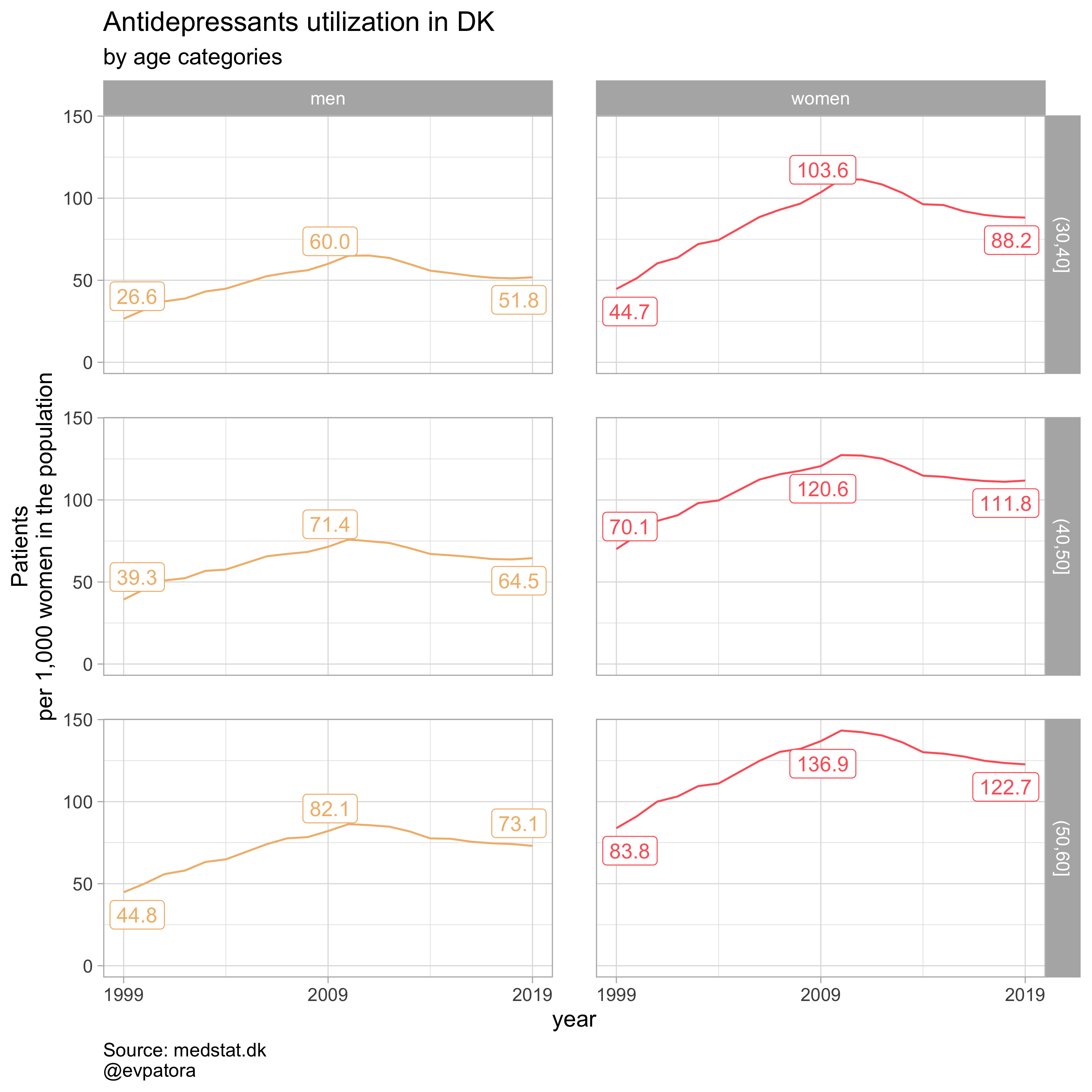
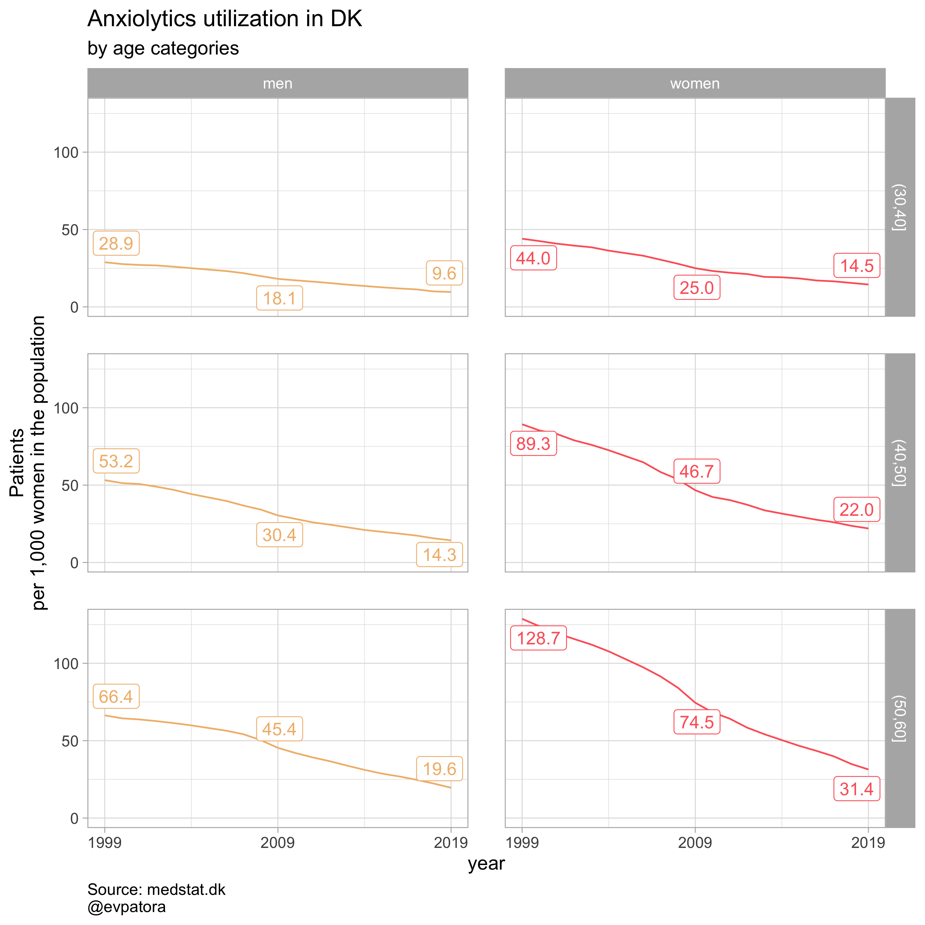
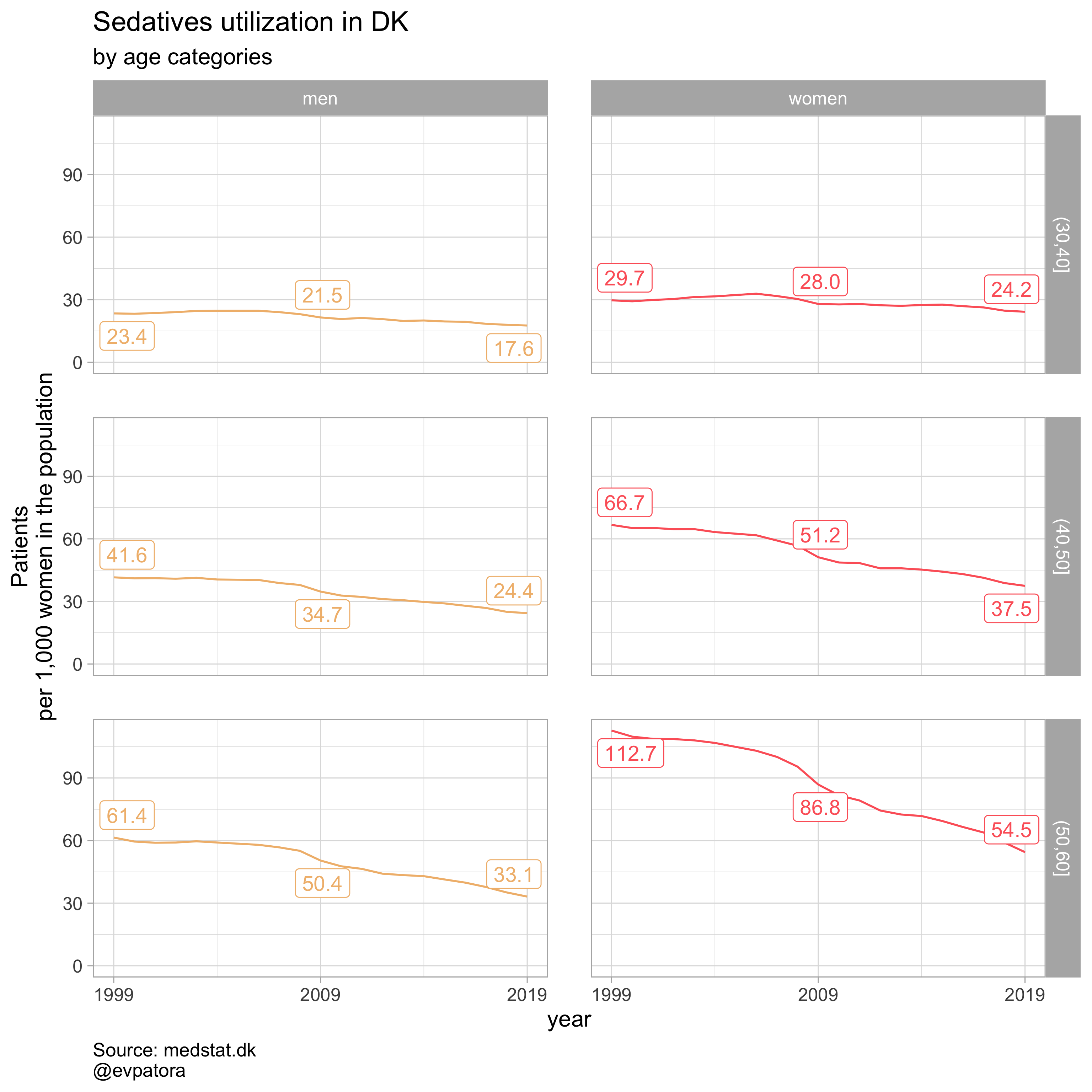
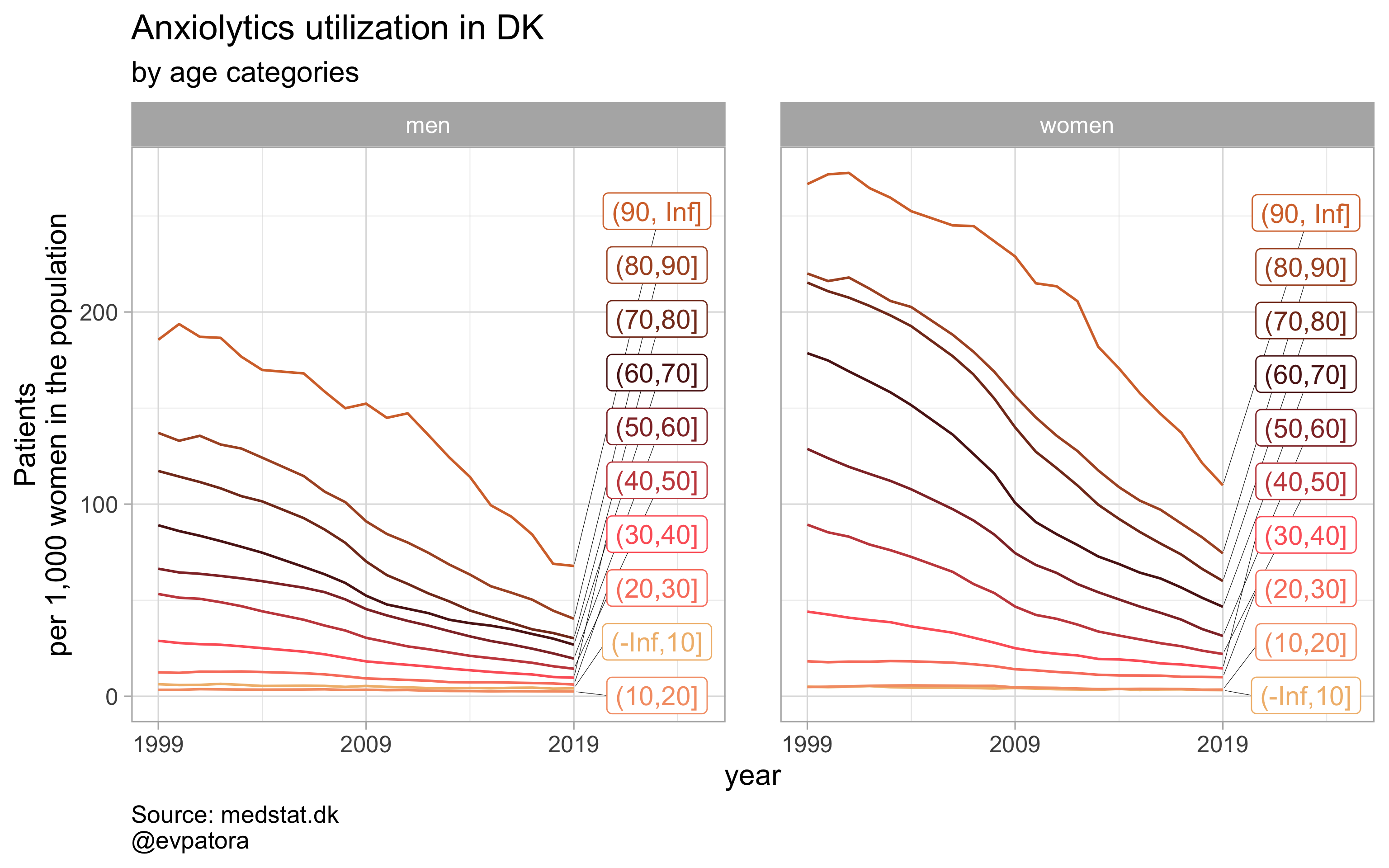
list_regex <- list(regex_antidepress, regex_antipsych, regex_anxiolyt, regex_sedat)
list_title <- list("Antidepressants", "Antipsychotics", "Anxiolytics", "Sedatives")
# iteration
list_plots <- map2(list_regex, list_title,
~plot_utilization_region(.my_data = data, atc = ATC, drug_regex = ..1,
age_var = age_cat, year_var = year, rate_var = patients_per_1000_inhabitants,
sex_var = gender_text, title = ..2))
list_plots
## [[1]]
##
## [[2]]

##
## [[3]]
##
## [[4]]
# can save all plots with one line
walk2(.x = list_plots, .y = list_title, ~ggsave(filename = paste0(Sys.Date(), "-", .y, ".pdf"),
                                                plot = .x, path = getwd(), device = cairo_pdf,
                                                width = 297, height = 210, units = "mm"))
Controling more than one variable in the custom function
Before we get to incorporate several more features to our customized plotting function, I want to include one intermediate step, where I will allow filtering the region column within the custom function. This will make it easier to plot a series of visualization for each of regions in addition to country-wide drug utilization rates in men and women. Note that I no longer select on specific age categories in this custom function as before.
# selected region, now all ages
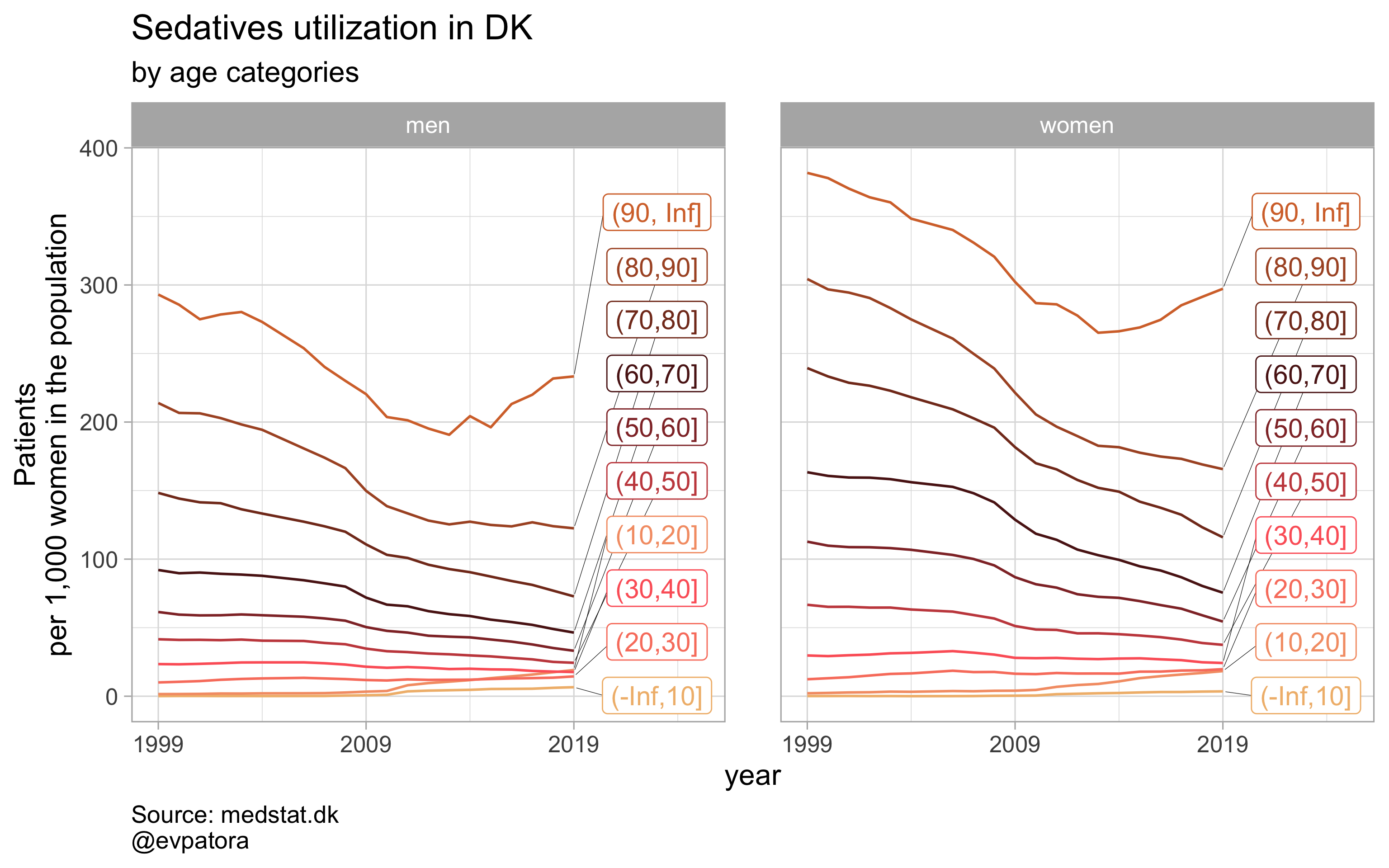
plot_utilization <- function(.my_data, drug_regex, atc, age_var, year_var, rate_var, sex_var, title, region_var, region_setting = "0"){
.my_data %>%
# I add the region_setting argument to my custom function, whose default would be a country level stats `region_setting = "0"`
filter({{ region_var }} == region_setting, str_detect({{ atc }}, drug_regex)) %>%
# make label for the year 2019
mutate(label = if_else({{ year_var }} == 2019, as.character(age_cat), NA_character_)) %>%
ggplot(aes(x = {{ year_var }}, y = {{ rate_var }}, color = {{ age_var }})) + # color now indicates age and not sex as before
geom_path() +
facet_grid(cols = vars({{ sex_var }}), scales = "fixed", drop = T) +
theme_light(base_size = 12) +
scale_x_continuous(limits = c(1999, 2025), breaks = c(seq(1999, 2019, 10))) +
expand_limits(y = 0) +
scale_color_manual(values = wes_palette(name = "GrandBudapest1", type = "continuous", n = 10)) +
ggrepel::geom_label_repel(aes(label = label), na.rm = TRUE, nudge_x = 4, direction = "y", segment.size = 0.1, segment.colour = "black", show.legend = F) +
theme(plot.caption = element_text(hjust = 0, size = 10),
legend.position = "none",
panel.spacing = unit(0.8, "cm")) +
labs(y = "Patients\nper 1,000 women in the population", title = paste0(title, " utilization in DK"), subtitle = "by age categories", caption = "Source: medstat.dk\n@evpatora")
}
# prepare the list to iterate along
list_regex <- list(regex_antidepress, regex_antipsych, regex_anxiolyt, regex_sedat)
list_title <- list("Antidepressants", "Antipsychotics", "Anxiolytics", "Sedatives")
# iteration
list_plots <- map2(list_regex, list_title,
~plot_utilization(.my_data = data, atc = ATC, drug_regex = ..1,
age_var = age_cat, year_var = year, rate_var = patients_per_1000_inhabitants,
sex_var = gender_text, title = ..2, region_var = region))
list_plots
## [[1]]
##
## [[2]]
##
## [[3]]
##
## [[4]]
# save all graphs with one line
walk2(.x = list_plots, .y = list_title, ~ggsave(filename = paste0(Sys.Date(), "-", .y, "_Syddanmark.pdf"),
                                                plot = .x, path = getwd(), device = cairo_pdf,
                                                width = 297, height = 210, units = "mm"))
Finalize customization based on your needs
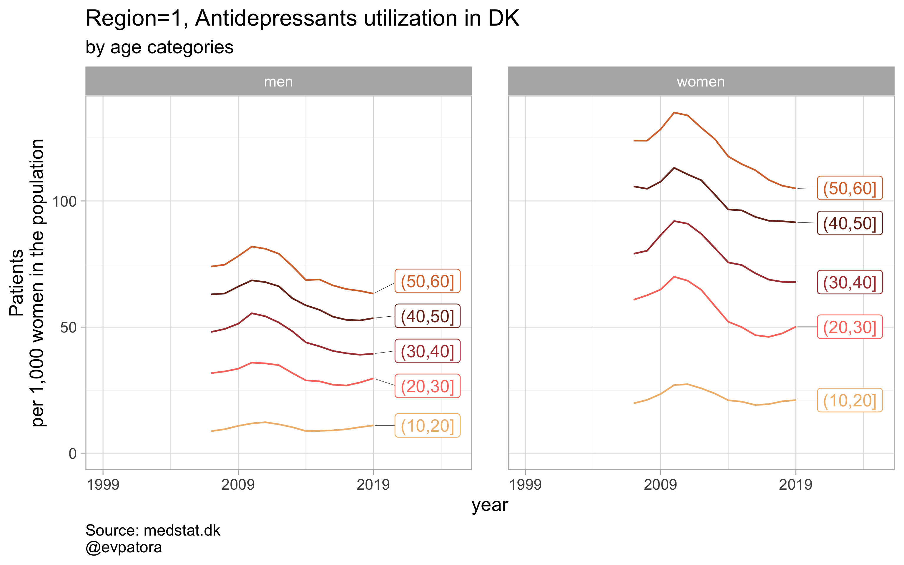
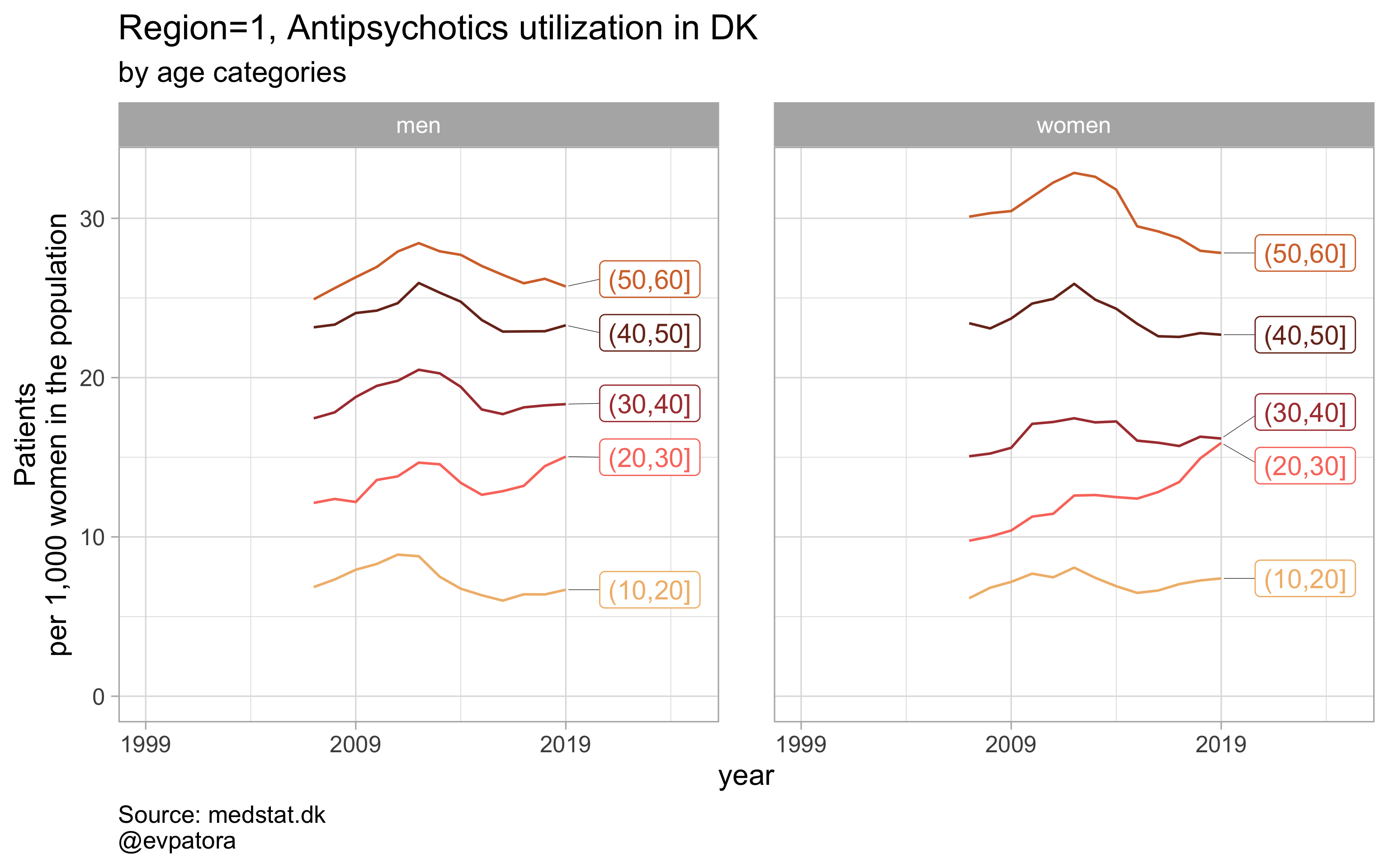
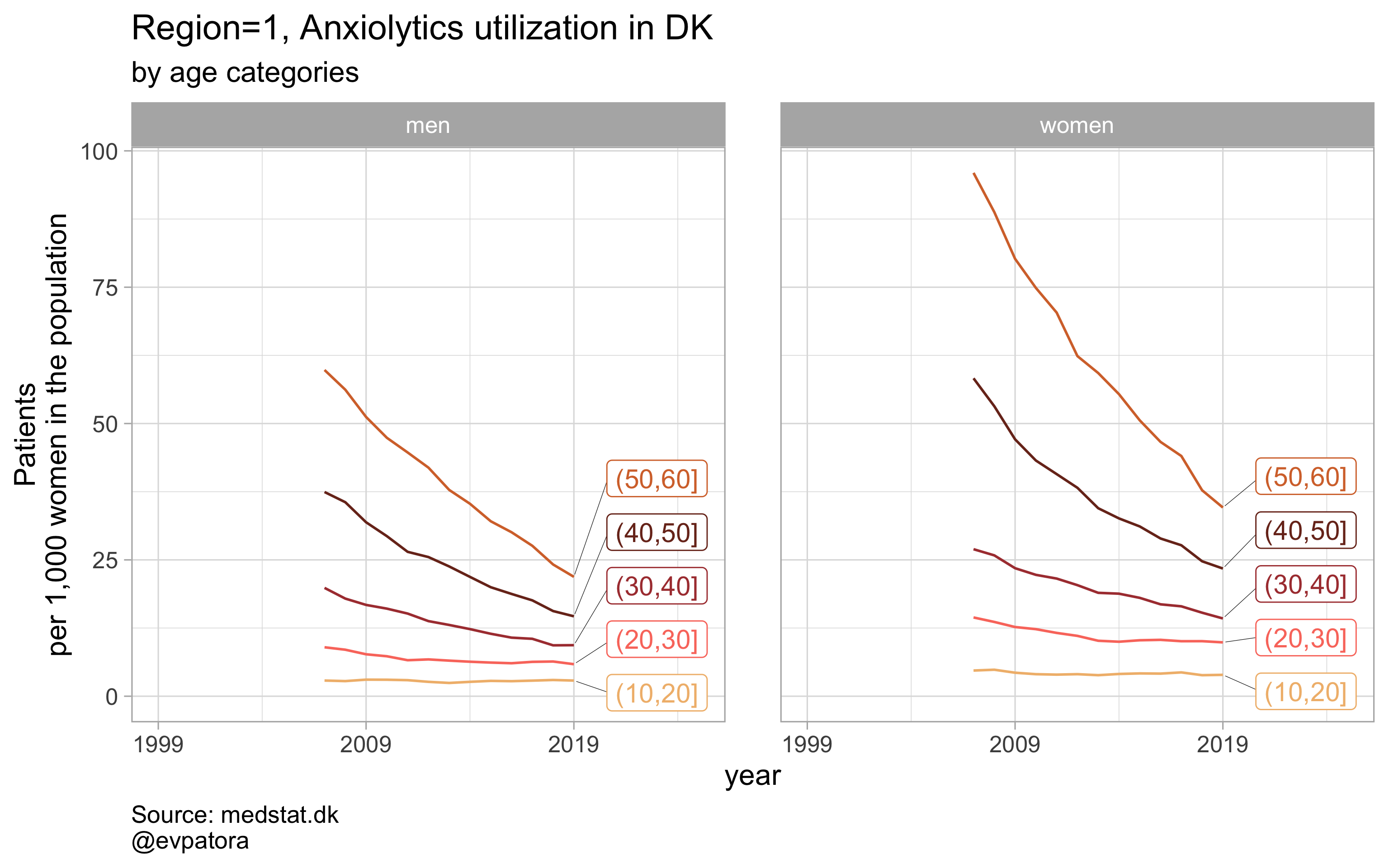
Now, I want to have control over age groups to be visualized. I will add a new argument age_setting into my custom function to implement this. Depending on what is my final goal, I can make a finalized function:
- For the visualization of selected drugs utilization rates in women vs men by age category explicitly (as many facets as selected age groups) or
- For visualization of selected drugs utilization rates in women vs men by age category implicitly (faceting data for women vs men and making no facets for age categories).
- For visualization of selected drugs utilization rates in women vs men by age category and by region on the same graph
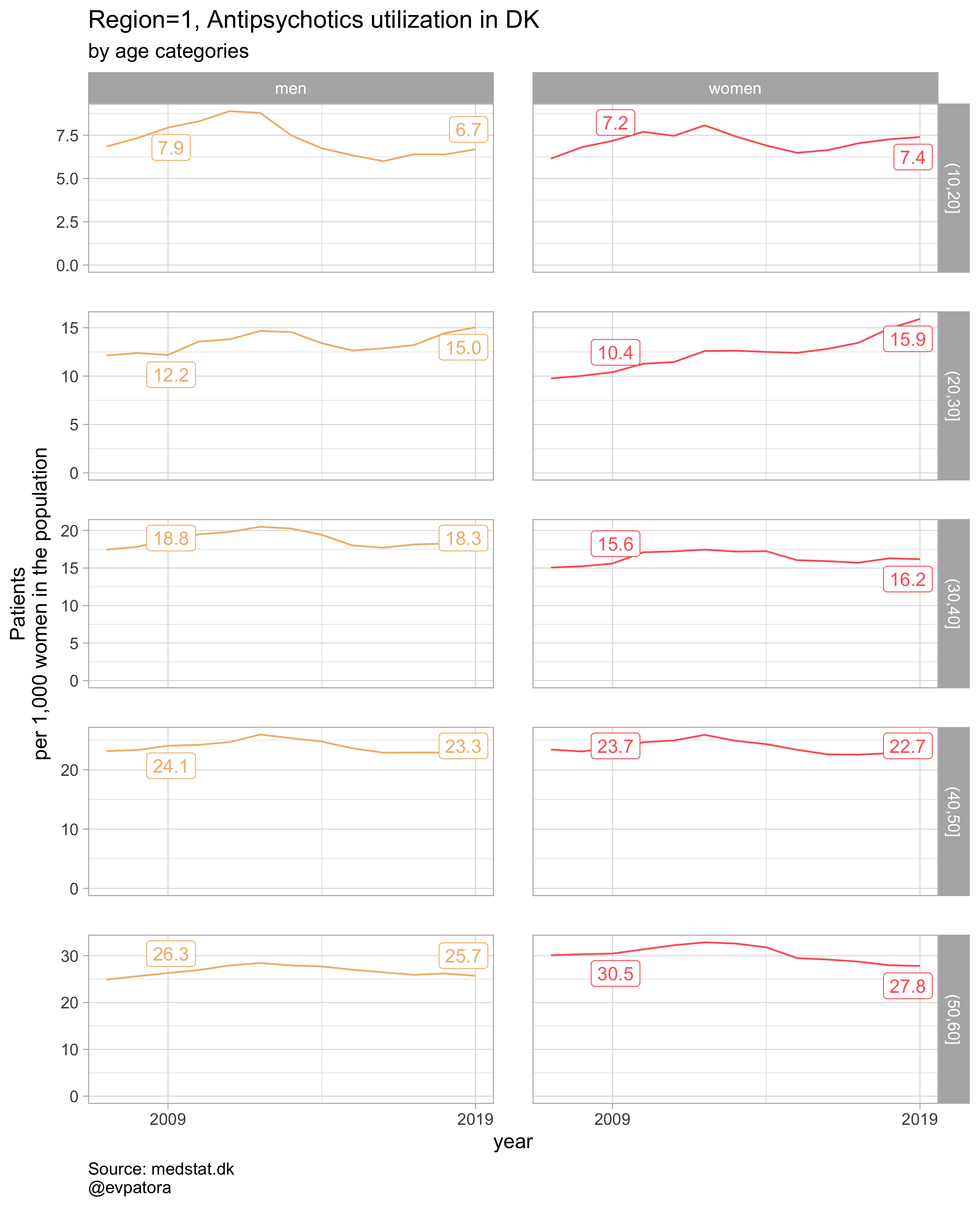
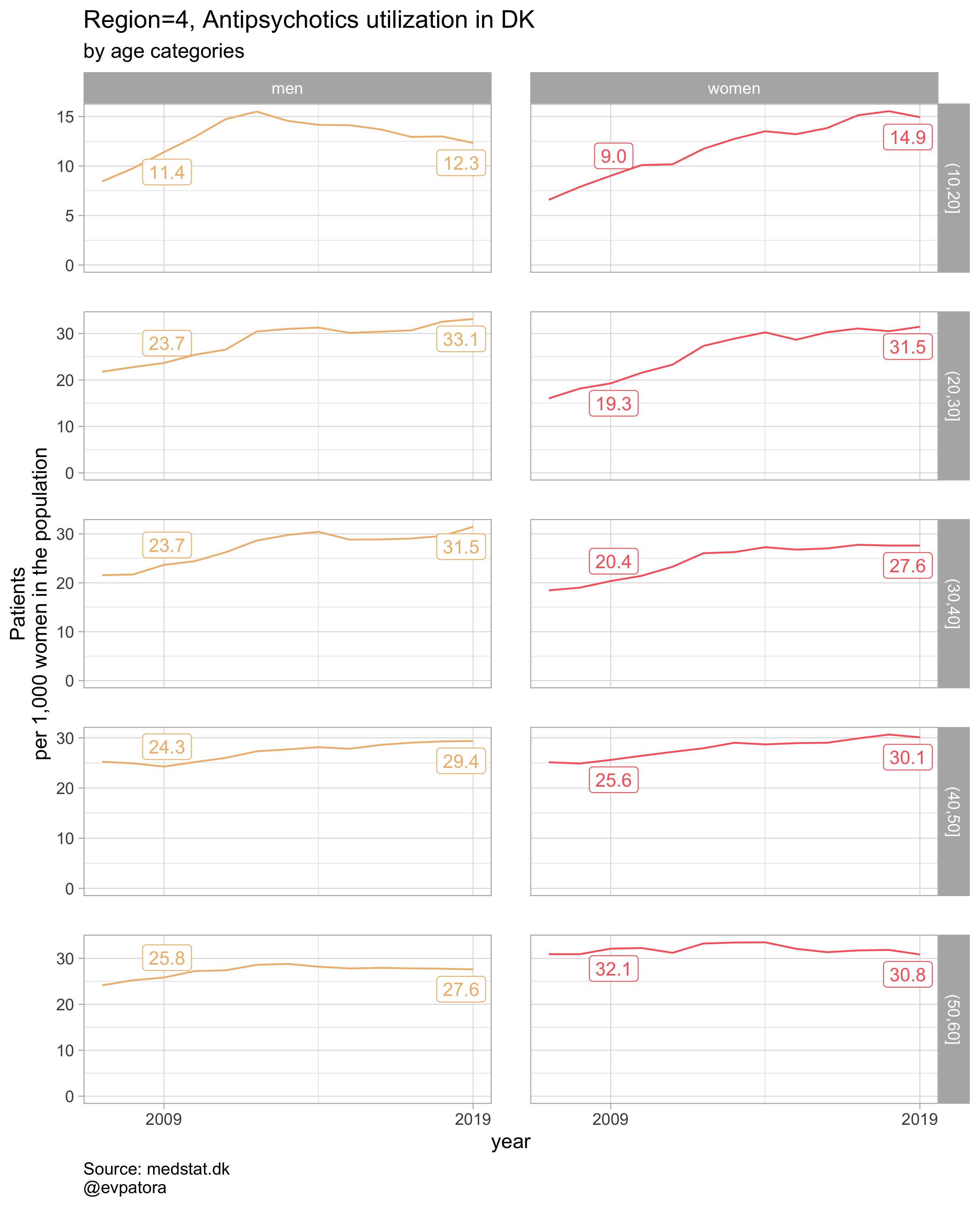
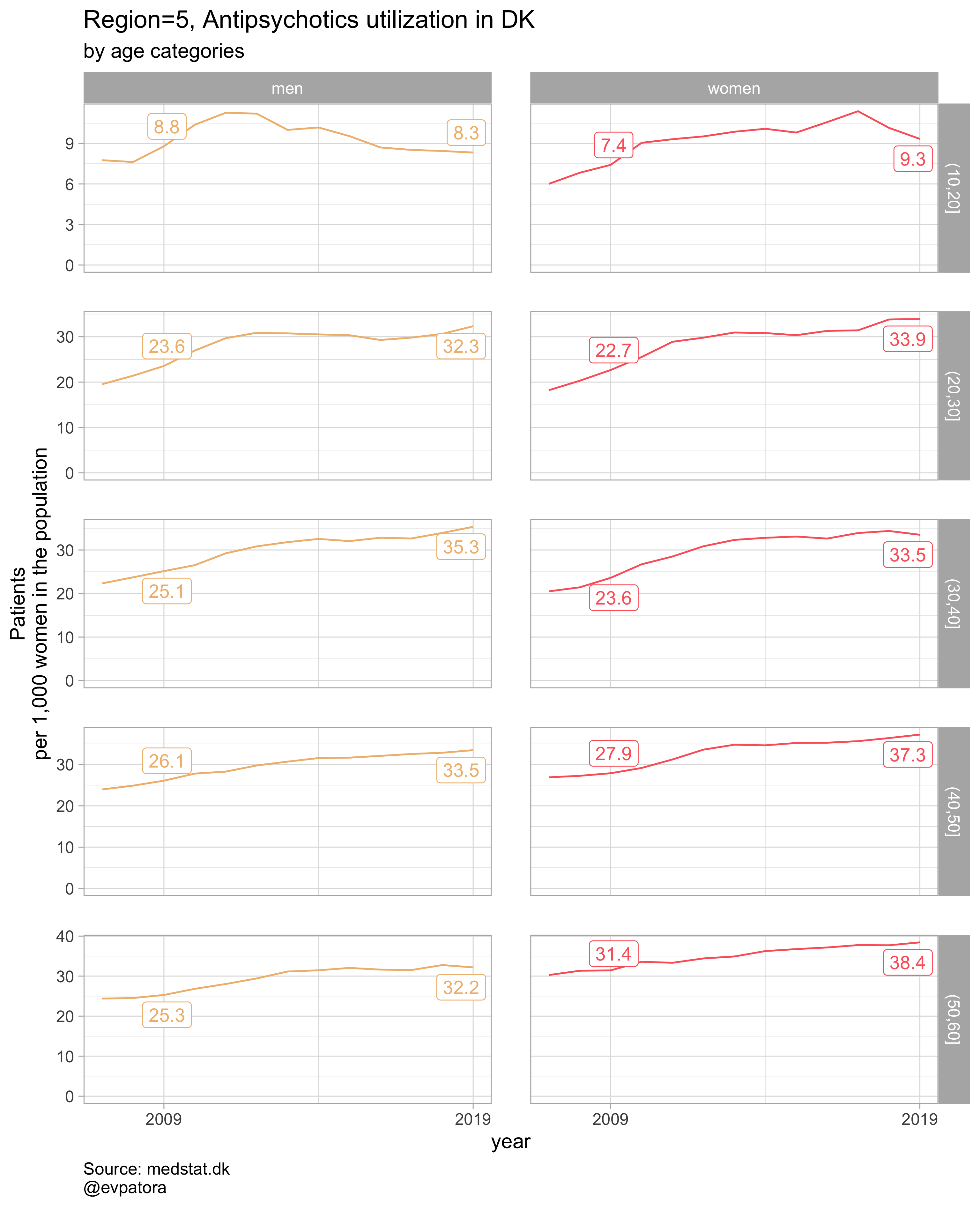
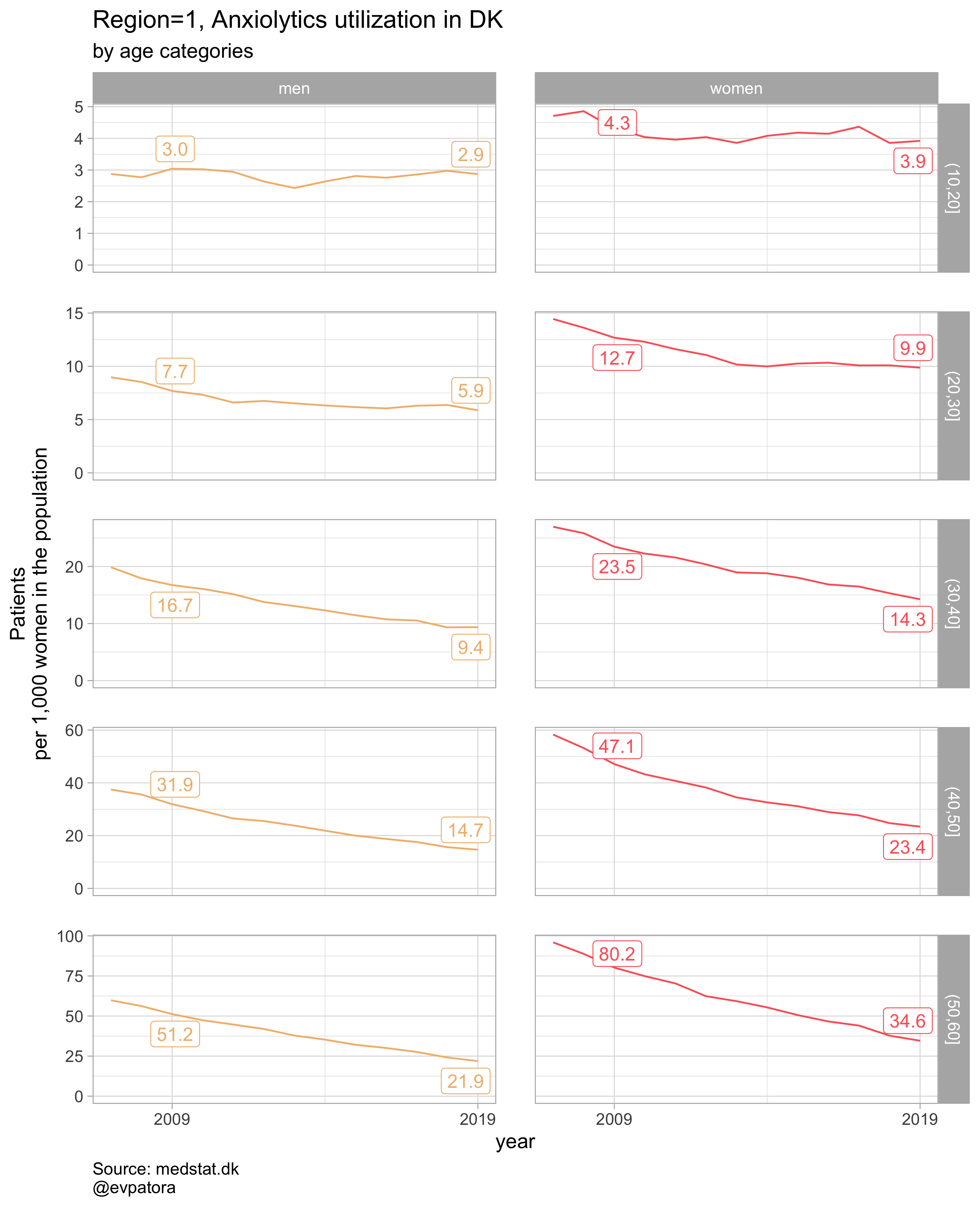
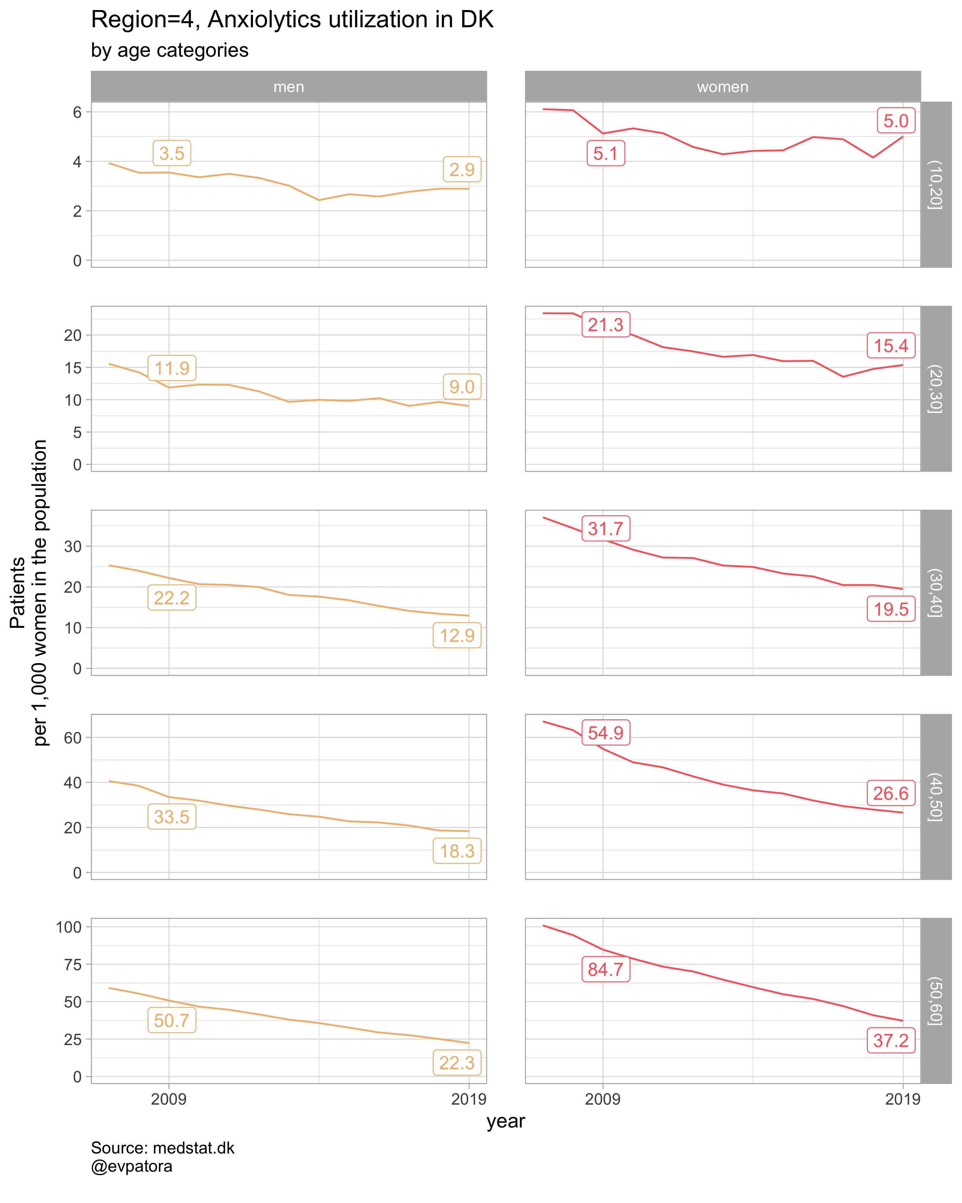
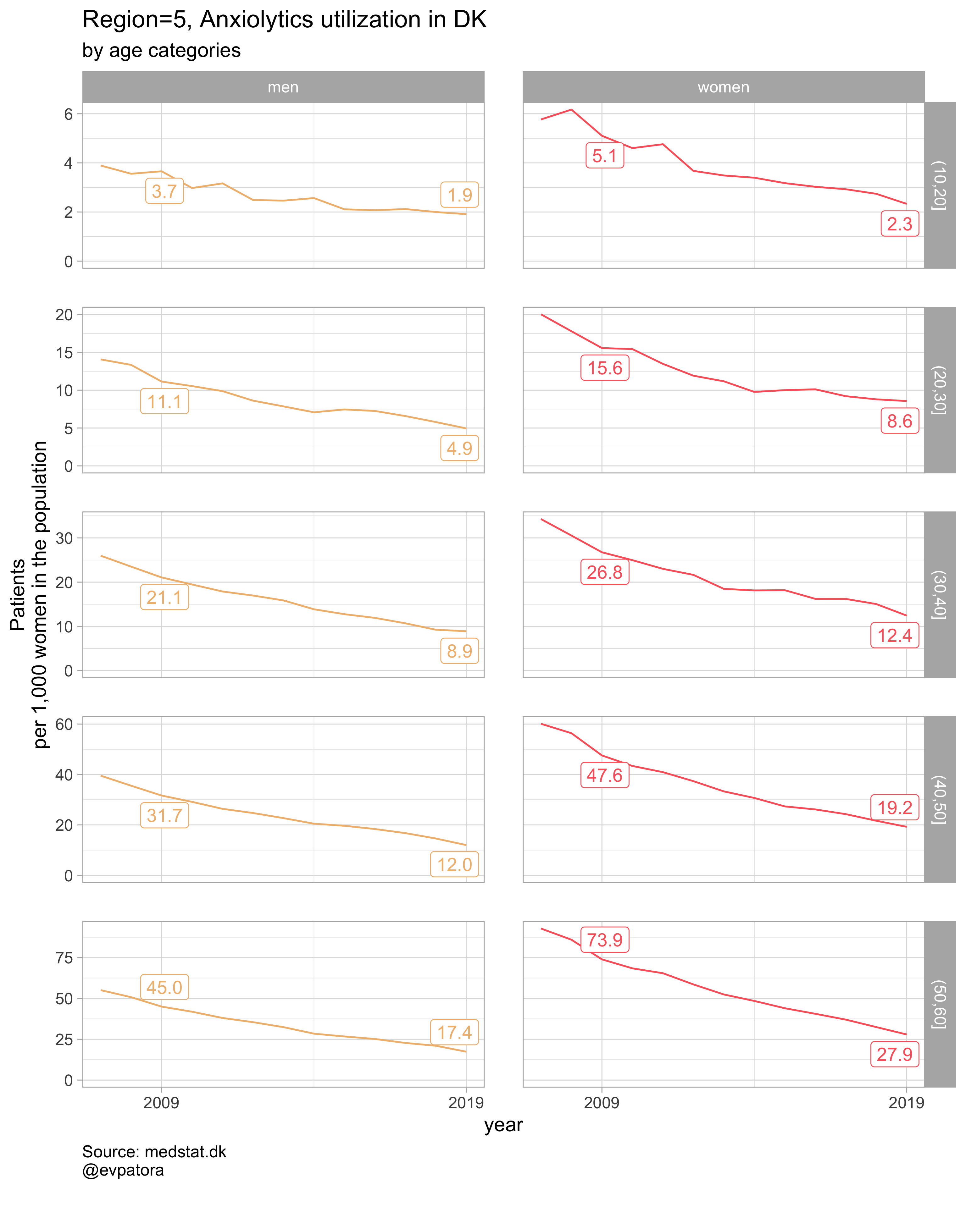
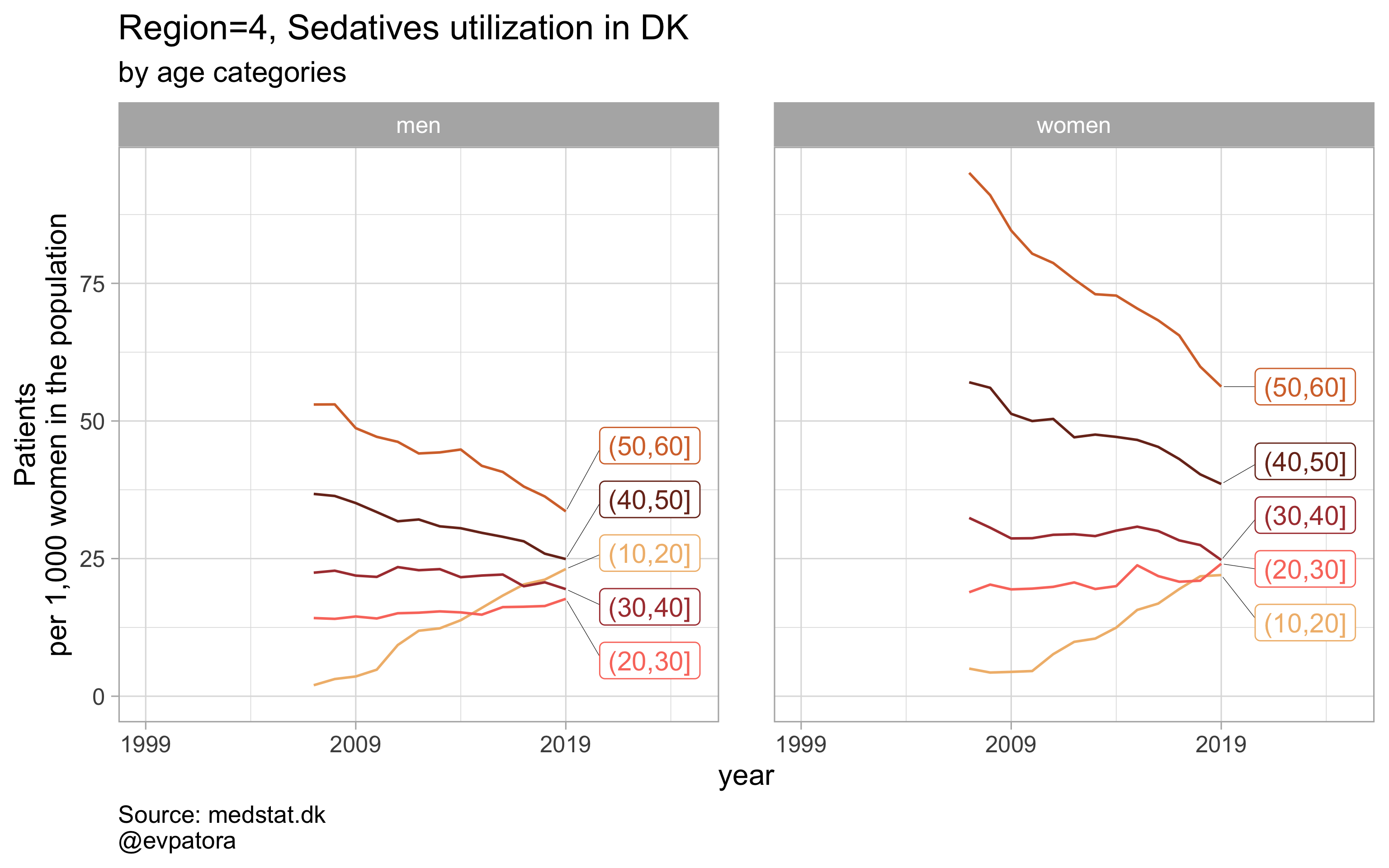
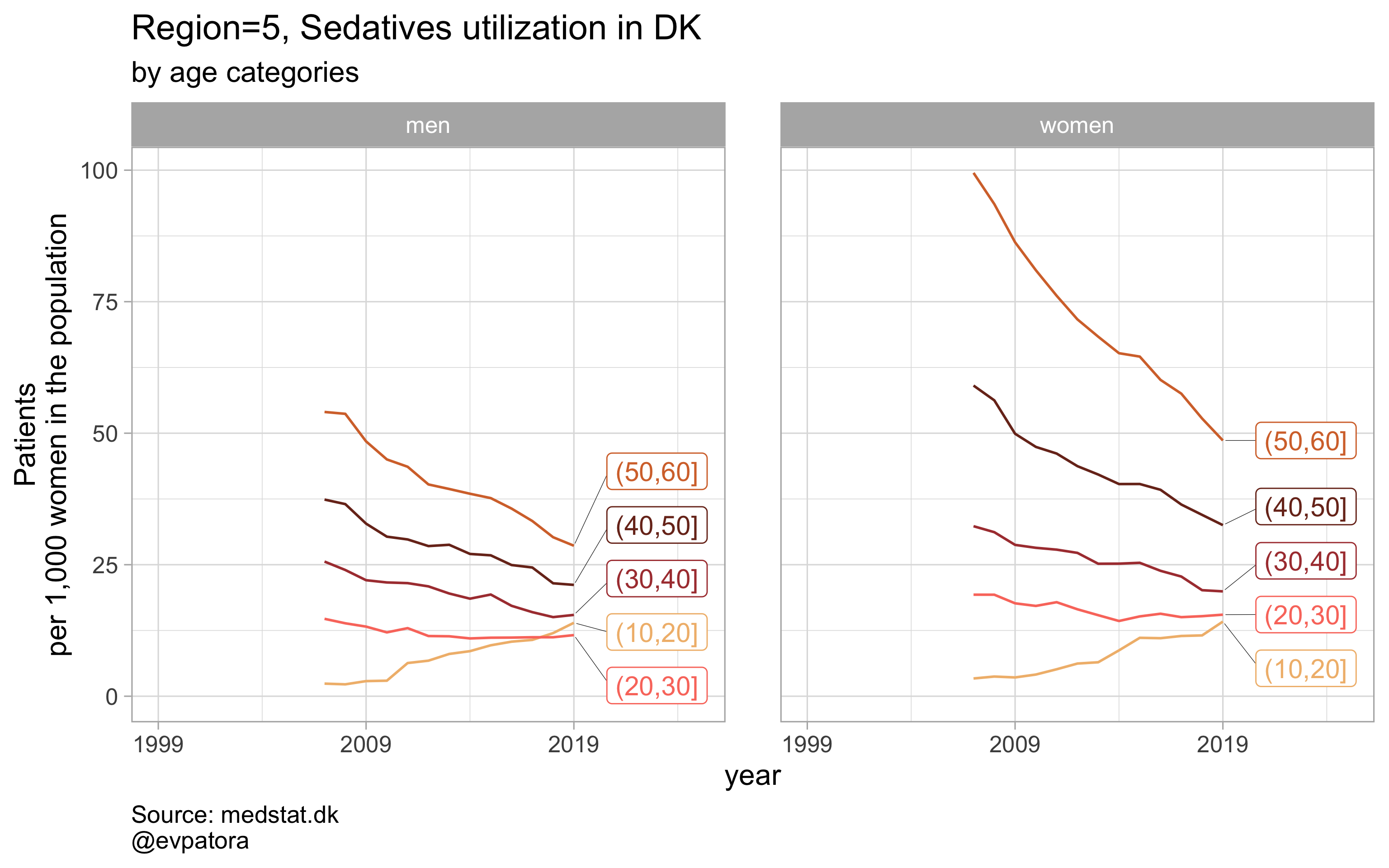
Option 1
NB! Some regions seem to miss data and in options 1 and 2 I do not explicitly exclude such regions
# for all regions & for selected age categories
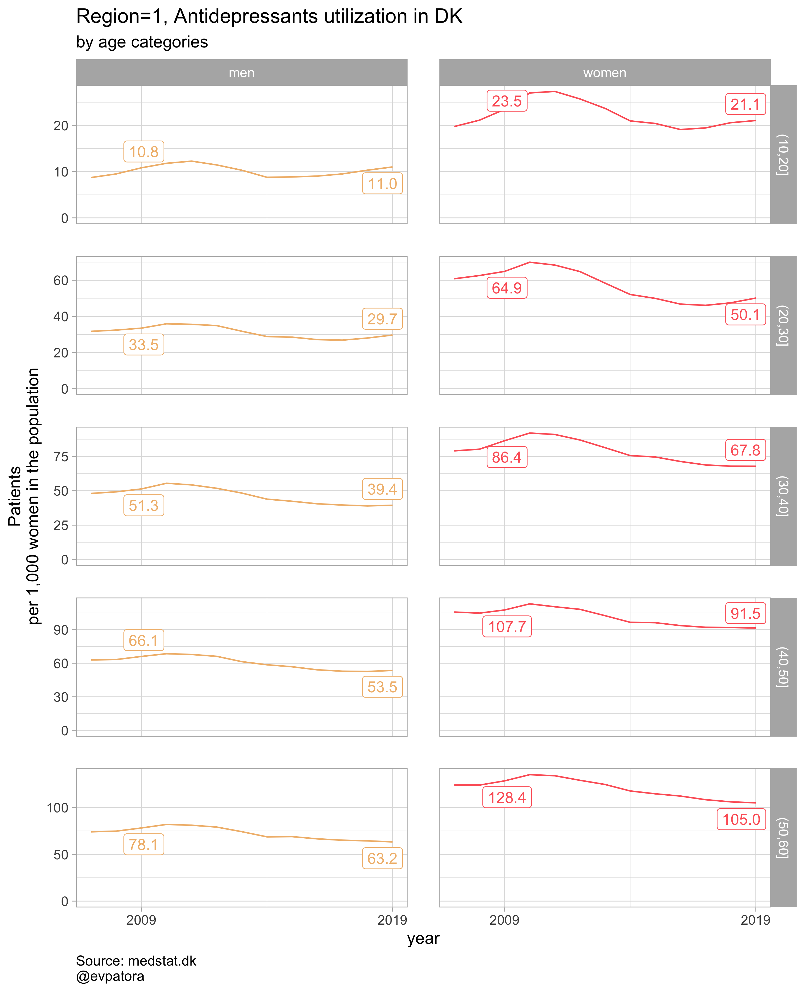
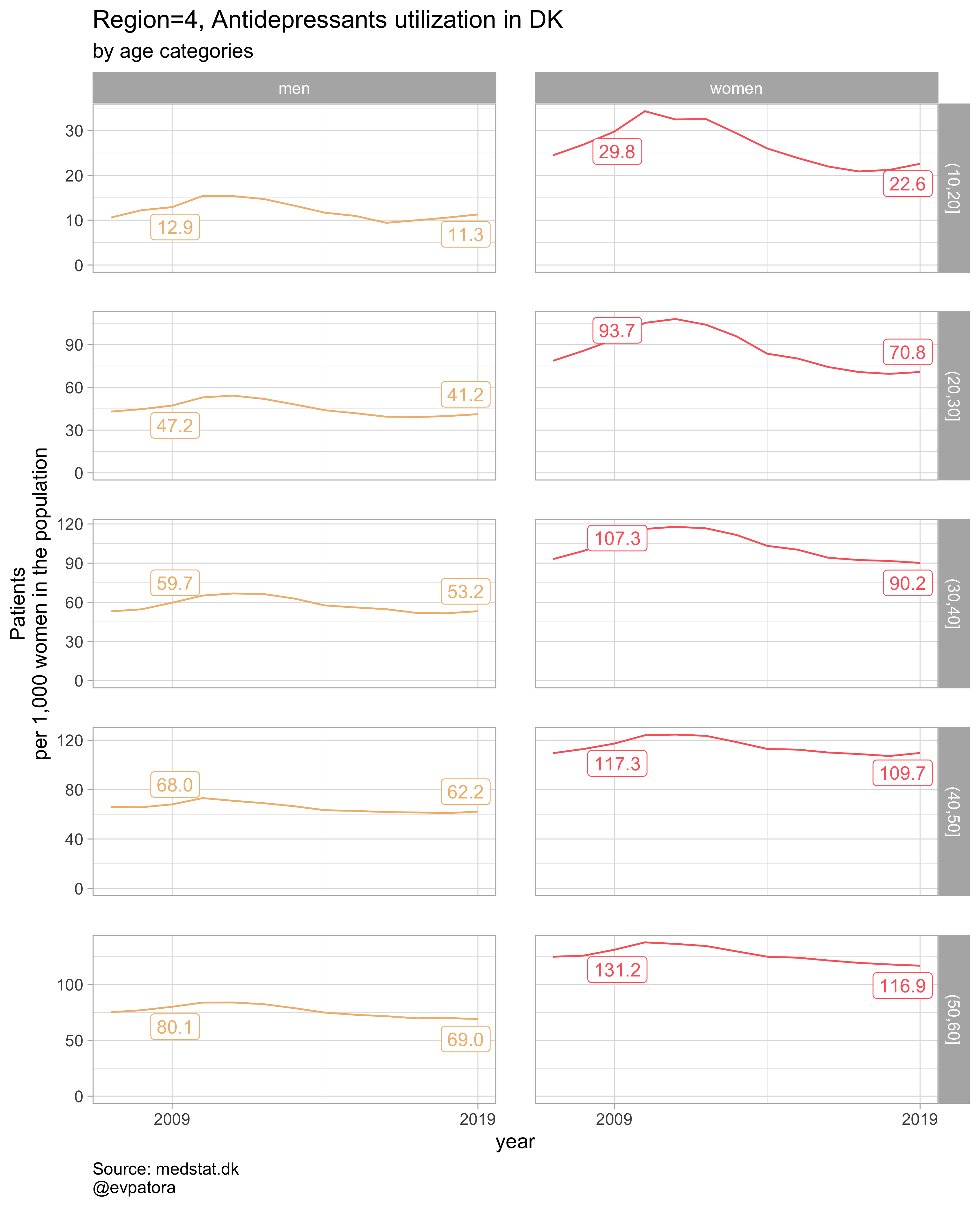
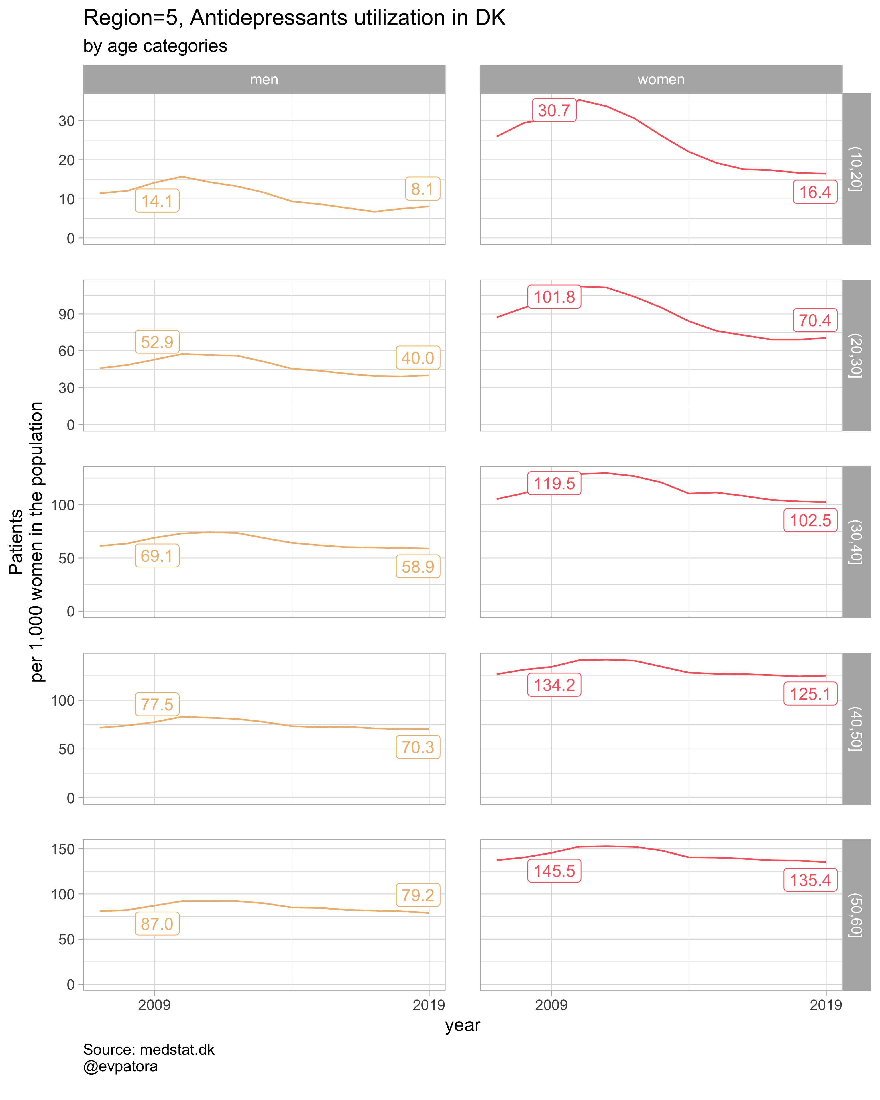
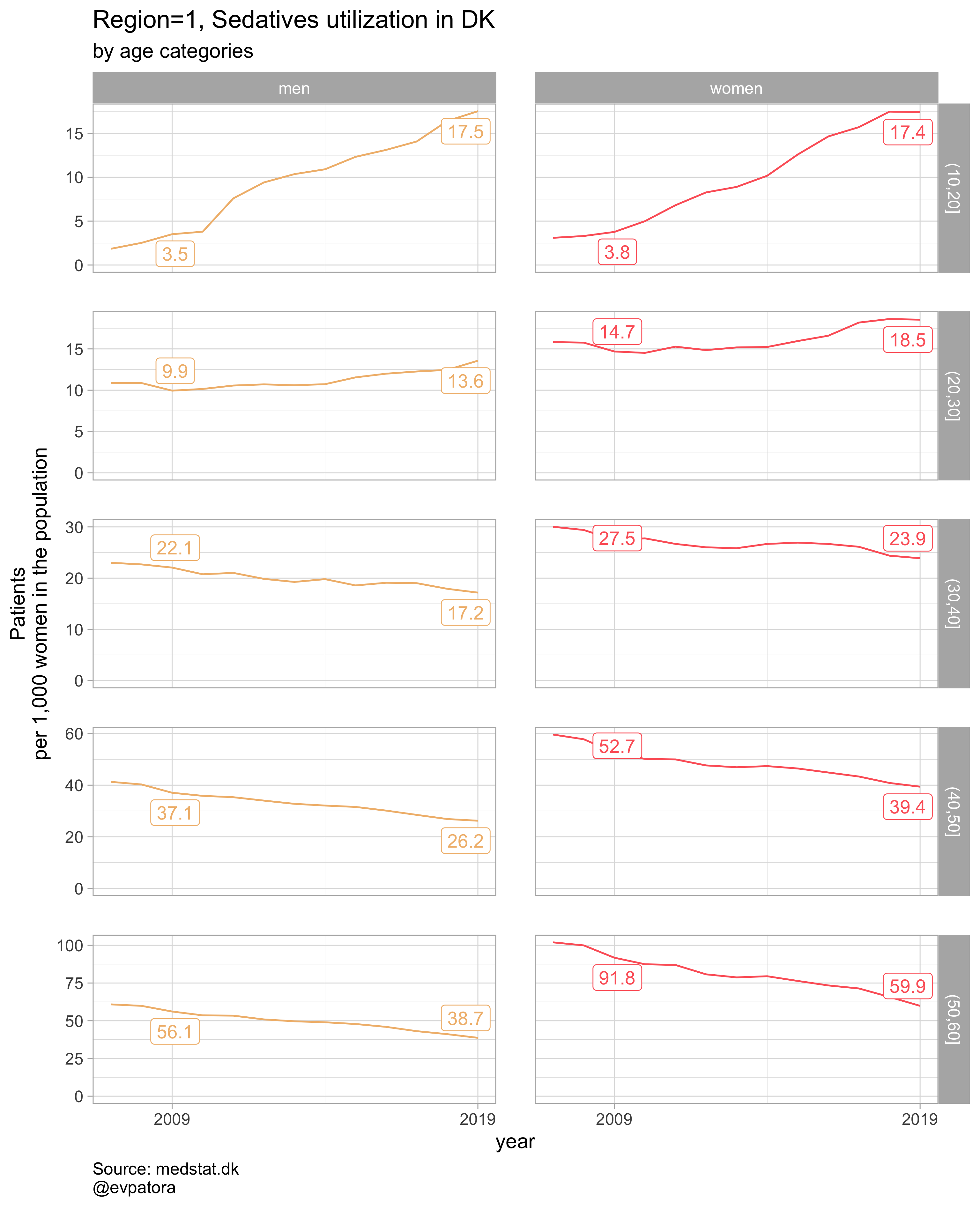
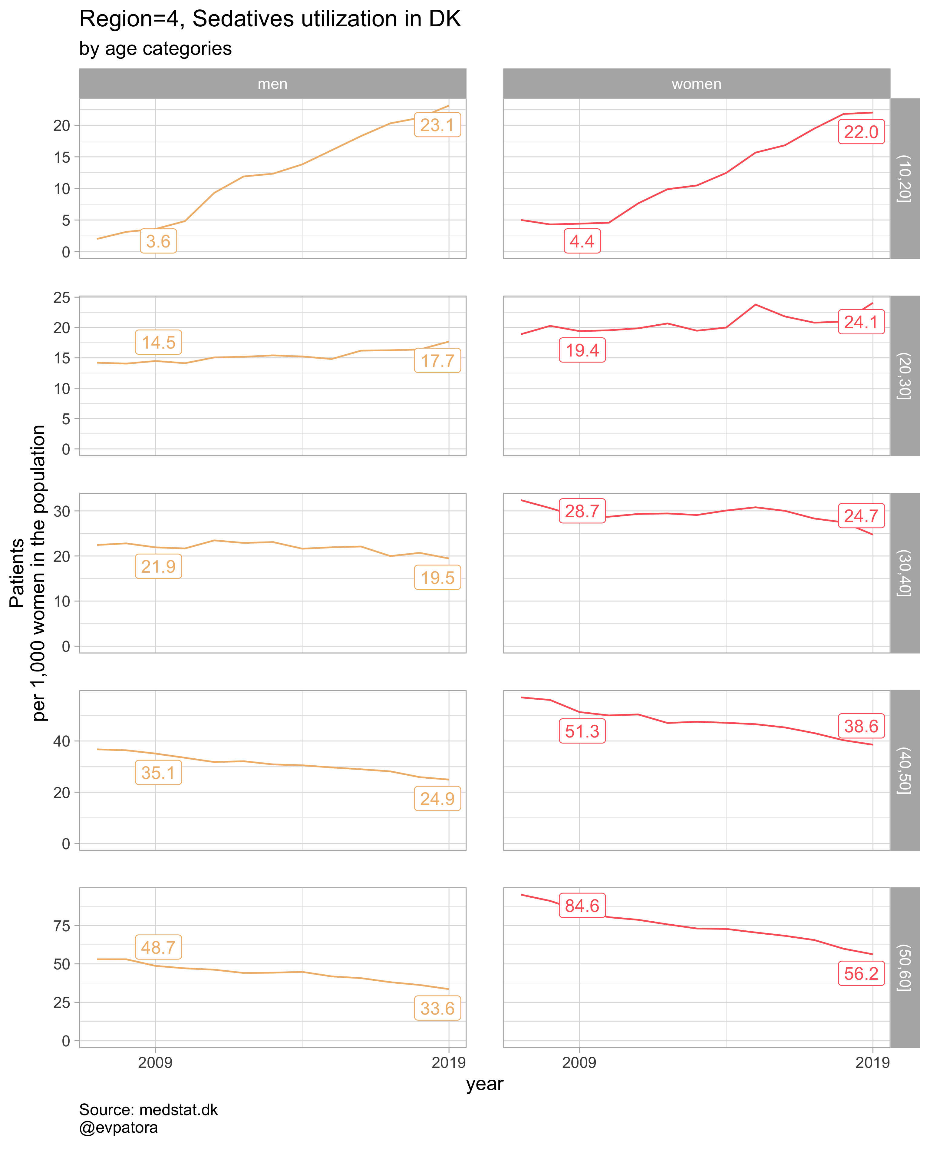
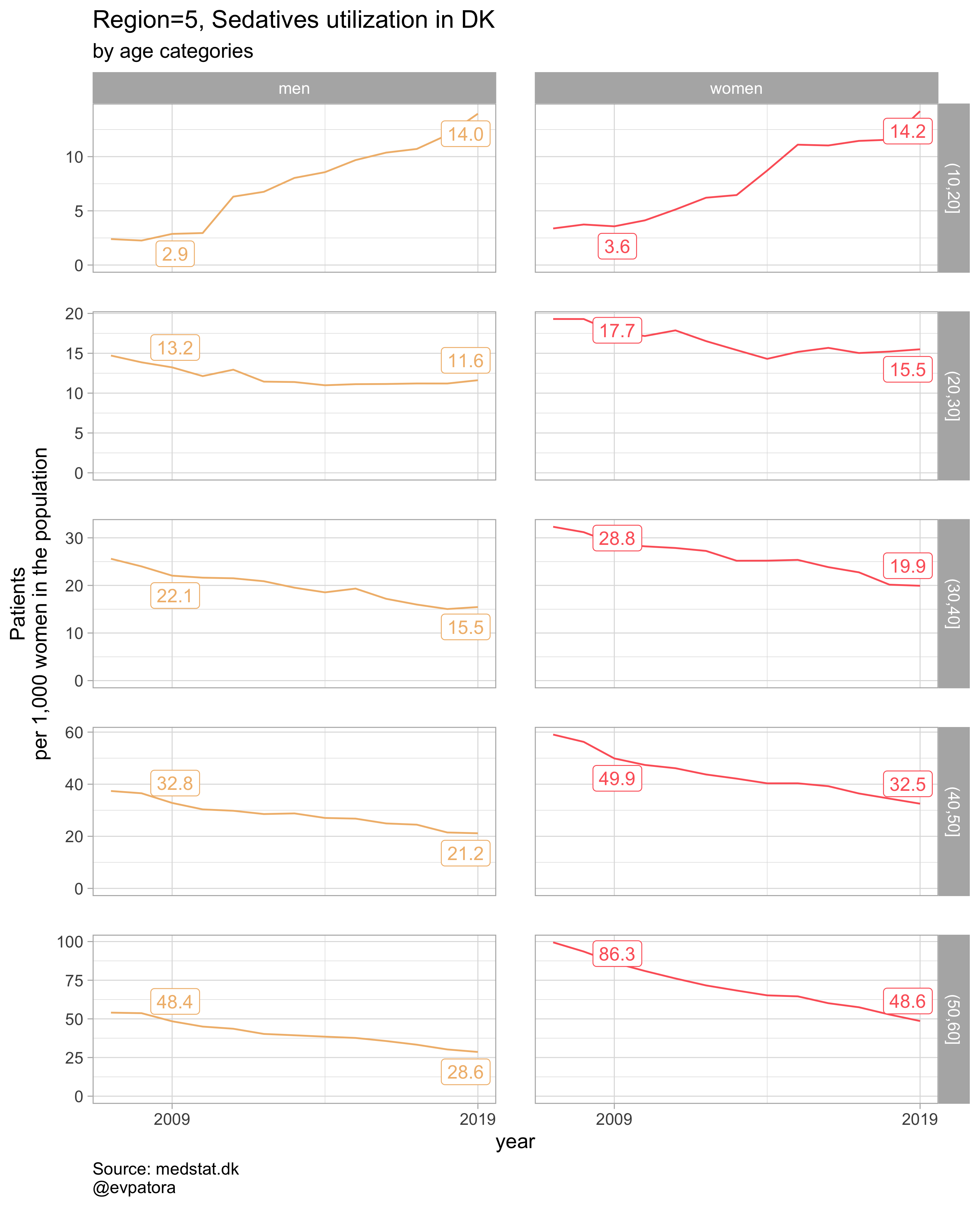
plot_utilization <- function(.my_data, drug_regex, atc, age_var, year_var, rate_var, sex_var, title, region_var, region_setting = "0", age_numeric, age_setting){
.my_data %>%
filter({{ age_numeric }} %in% age_setting, {{ region_var }} == region_setting, str_detect({{ atc }}, drug_regex)) %>%
mutate(
label = if_else({{ year_var }} == 1999 | {{ year_var }} == 2009 | {{ year_var }} == 2019, as.character(sprintf("%1.1f", round({{ rate_var }}, digits = 1))), NA_character_)
) %>%
ggplot(aes(x = {{ year_var }}, y = {{ rate_var }}, color = {{ sex_var }})) +
geom_path() +
facet_grid(cols = vars({{ sex_var }}), rows = vars({{ age_var }}), scales = "free", drop = T) +
theme_light(base_size = 12) +
scale_x_continuous(breaks = c(seq(1999, 2019, 10))) +
expand_limits(y = 0) +
ggrepel::geom_label_repel(aes(label = label), na.rm = TRUE, nudge_x = 0.1, direction = "y", segment.size = 0.1, segment.colour = "black", show.legend = F) +
theme(plot.caption = element_text(hjust = 0, size = 10),
legend.position = "none",
panel.spacing = unit(0.8, "cm")) +
scale_color_manual(values = wes_palette(name = "GrandBudapest1", type = "discrete")) +
theme(plot.caption = element_text(hjust = 0, size = 10),
legend.position = "none",
panel.spacing = unit(0.8, "cm")) +
labs(y = "Patients\nper 1,000 women in the population", title = paste0(title, " utilization in DK"), subtitle = "by age categories", caption = "Source: medstat.dk\n@evpatora\n")
}
# 4 drugs for 5 regions = 20 elements
list_region <- list(1:5) %>% map(~as.character(.x)) %>% rep(times = 4) %>% flatten()
list_regex <- list(regex_antidepress, regex_antipsych, regex_anxiolyt, regex_sedat) %>% rep(each = 5)
list_drug_name <- list("Antidepressants", "Antipsychotics", "Anxiolytics", "Sedatives") %>% rep(each = 5)
list_title <- map2(list_region, list_drug_name, ~paste0("Region=", .x, ", ", .y))
# iteration
list_plots <- pmap(.l = list(list_regex, list_title, list_region),
.f = ~plot_utilization(.my_data = data, atc = ATC, drug_regex = ..1,
age_var = age_cat, year_var = year, rate_var = patients_per_1000_inhabitants,
sex_var = gender_text, title = ..2, region_var = region, region_setting = ..3,
age_numeric = age, age_setting = 10:60))
# see some results
list_plots
## [[1]]
##
## [[2]]

##
## [[3]]

##
## [[4]]
##
## [[5]]
##
## [[6]]
##
## [[7]]
##
## [[8]]

##
## [[9]]
##
## [[10]]
##
## [[11]]
##
## [[12]]
##
## [[13]]

##
## [[14]]
##
## [[15]]
##
## [[16]]
##
## [[17]]
##
## [[18]]

##
## [[19]]
##
## [[20]]
# save all plots with one line: each saved plot has the name of the parameters plotted (medication & region)
walk2(.x = list_plots, .y = list_title, ~ggsave(filename = paste0(Sys.Date(), "-", .y, ".pdf"),
                                                plot = .x, path = getwd(), device = cairo_pdf,
                                                width = 297, height = 210, units = "mm"))
Option 2
# for all regions & for selected age categories no age facets
plot_utilization <- function(.my_data, drug_regex, atc, age_var, year_var, rate_var, sex_var, title, region_var, region_setting = "0", age_numeric, age_setting, n = 5){
  .my_data %>%
    filter({{ age_numeric }} %in% age_setting, {{ region_var }} == region_setting, str_detect({{ atc }}, drug_regex)) %>%
    # make label for the year 2019
    mutate(label = if_else({{ year_var }} == 2019, as.character(age_cat), NA_character_)) %>%
    ggplot(aes(x = {{ year_var }}, y = {{ rate_var }}, color = {{ age_var }})) +
    geom_path() +
    facet_grid(cols = vars({{ sex_var }}), scales = "free", drop = T) +
    theme_light(base_size = 12) +
    scale_x_continuous(limits = c(1999, 2025), breaks = c(seq(1999, 2019, 10))) +
    expand_limits(y = 0) +
    scale_color_manual(values = wes_palette(name = "GrandBudapest1", type = "continuous", n = n)) +
    ggrepel::geom_label_repel(aes(label = label), na.rm = TRUE, nudge_x = 4, direction = "y", segment.size = 0.1, segment.colour = "black", show.legend = F) +
    theme(plot.caption = element_text(hjust = 0, size = 10),
          legend.position = "none",
          panel.spacing = unit(0.8, "cm")) +
    labs(y = "Patients\nper 1,000 women in the population", title = paste0(title, " utilization in DK"), subtitle = "by age categories", caption = "Source: medstat.dk\n@evpatora")
}

# 4 drugs for 5 regions = 20 elements
list_region <- list(1:5) %>% map(~as.character(.x)) %>% rep(times = 4) %>% flatten() # this is not pretty, but it works :)
list_regex <- list(regex_antidepress, regex_antipsych, regex_anxiolyt, regex_sedat) %>% rep(each = 5)
list_drug_name <- list("Antidepressants", "Antipsychotics", "Anxiolytics", "Sedatives") %>% rep(each = 5)
list_title <- map2(list_region, list_drug_name, ~paste0("Region=", .x, ", ", .y))

# iteration
list_plots <- pmap(.l = list(list_regex, list_title, list_region),
                   .f = ~plot_utilization(.my_data = data, atc = ATC, drug_regex = ..1, # list_regex
                                          age_var = age_cat, year_var = year, rate_var = patients_per_1000_inhabitants,
                                          sex_var = gender_text, title = ..2, region_var = region, # list_title
                                          region_setting = ..3, age_numeric = age, age_setting = 10:60)) # list_region

# see some results
list_plots
## [[1]]
##
## [[2]]

##
## [[3]]
##
## [[4]]
##
## [[5]]
##
## [[6]]
##
## [[7]]

##
## [[8]]
##
## [[9]]
##
## [[10]]
##
## [[11]]
##
## [[12]]

##
## [[13]]
##
## [[14]]
##
## [[15]]
##
## [[16]]

##
## [[17]]

##
## [[18]]
##
## [[19]]
##
## [[20]]
# save all plots with one line: each saved plot has the name of the parameters plotted (medication & region)
walk2(.x = list_plots, .y = list_title, ~ggsave(filename = paste0(Sys.Date(), "-", .y, ".pdf"),
                                                plot = .x, path = getwd(), device = cairo_pdf,
                                                width = 297, height = 210, units = "mm"))
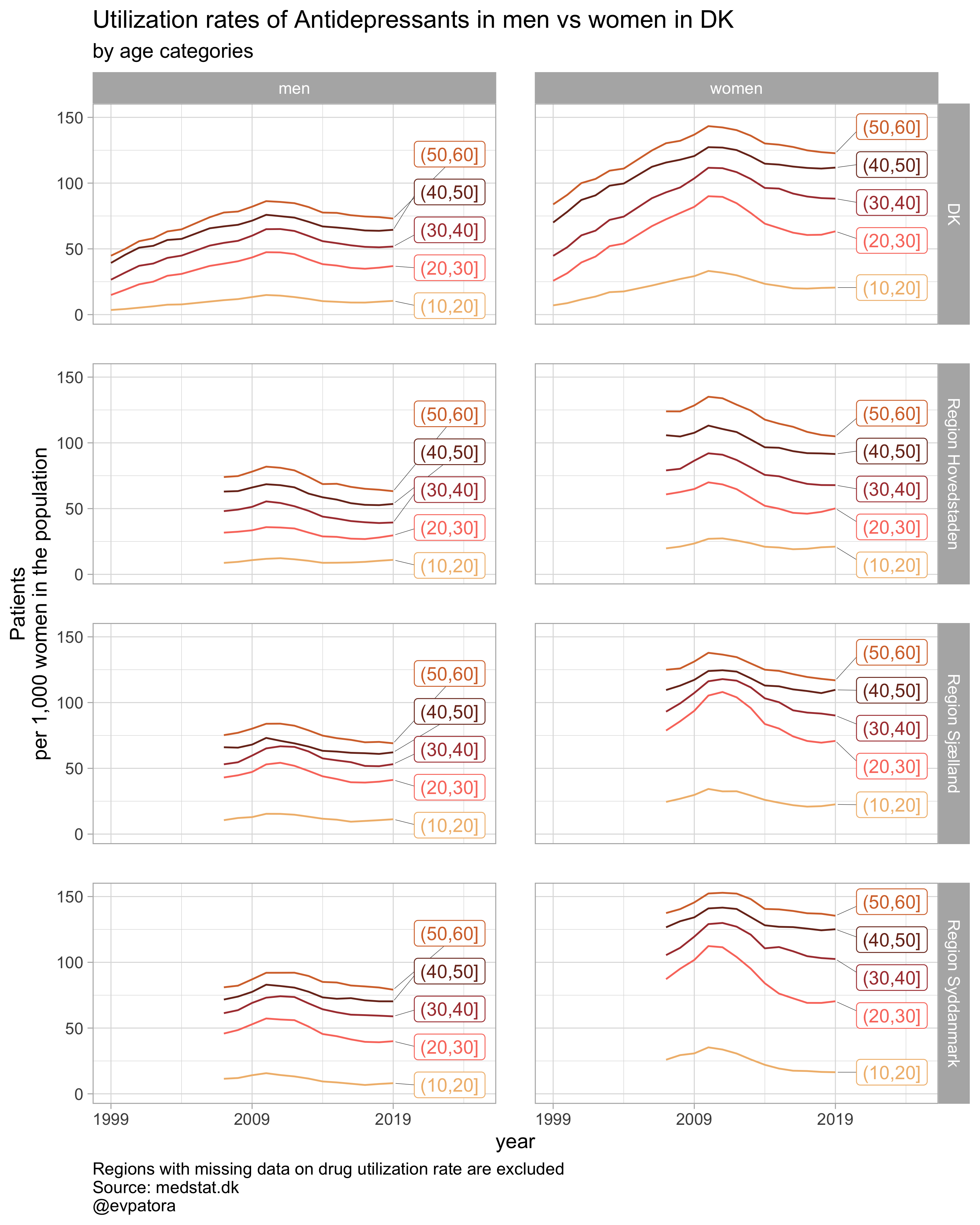
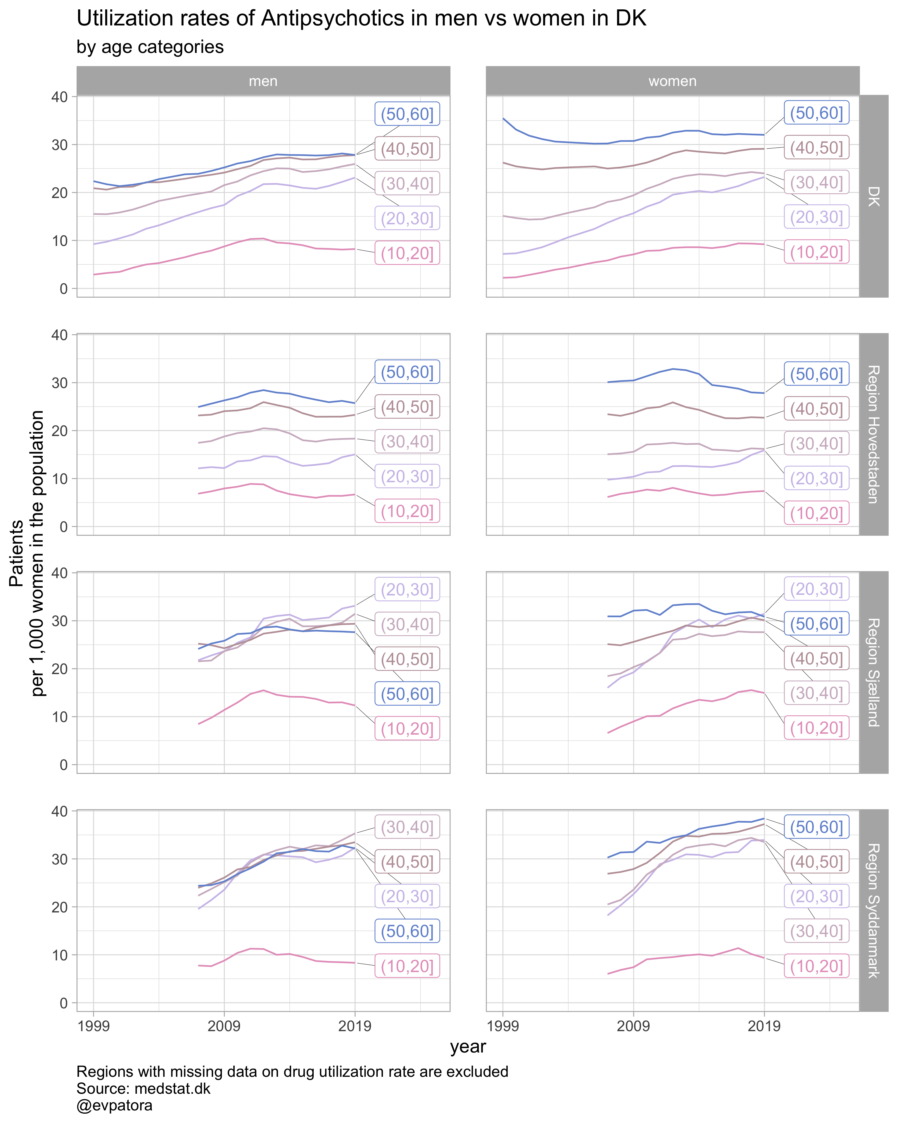
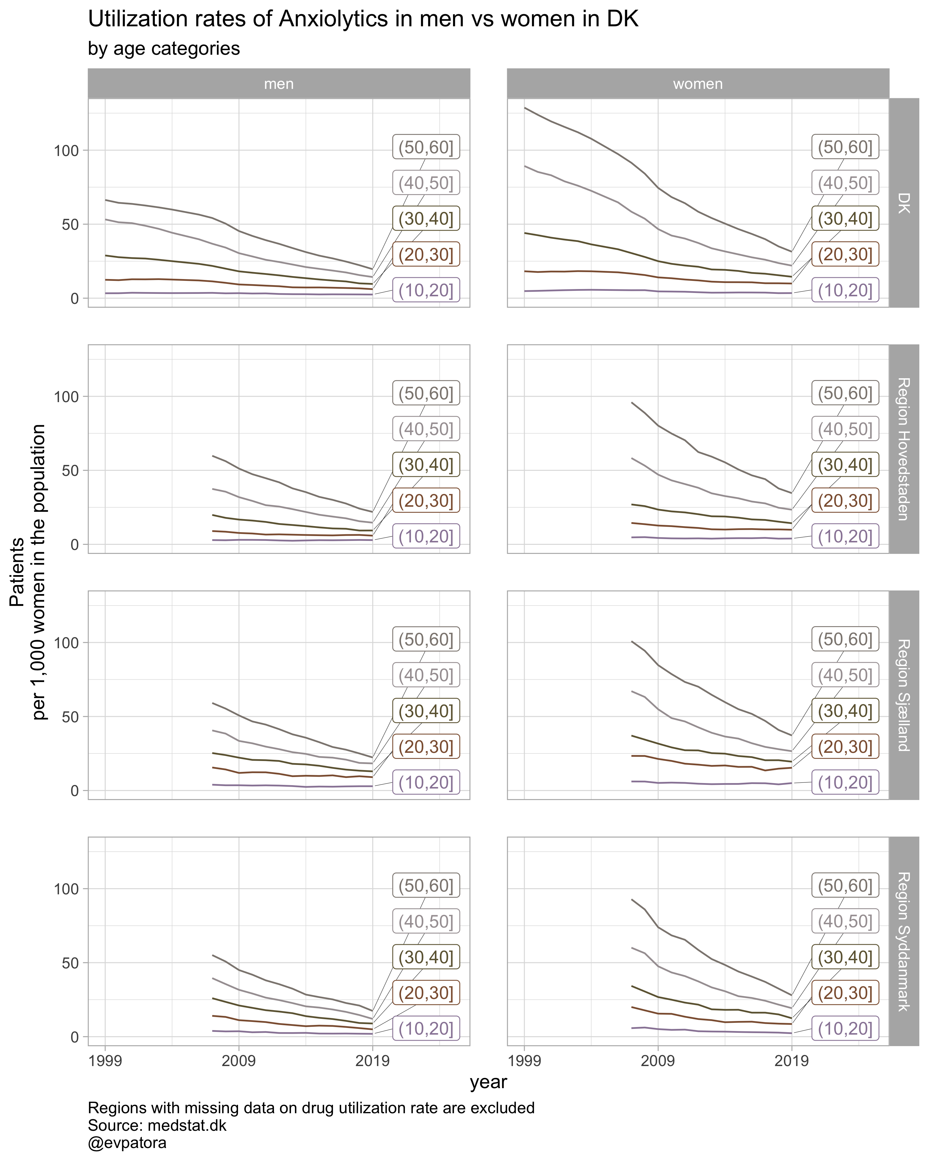
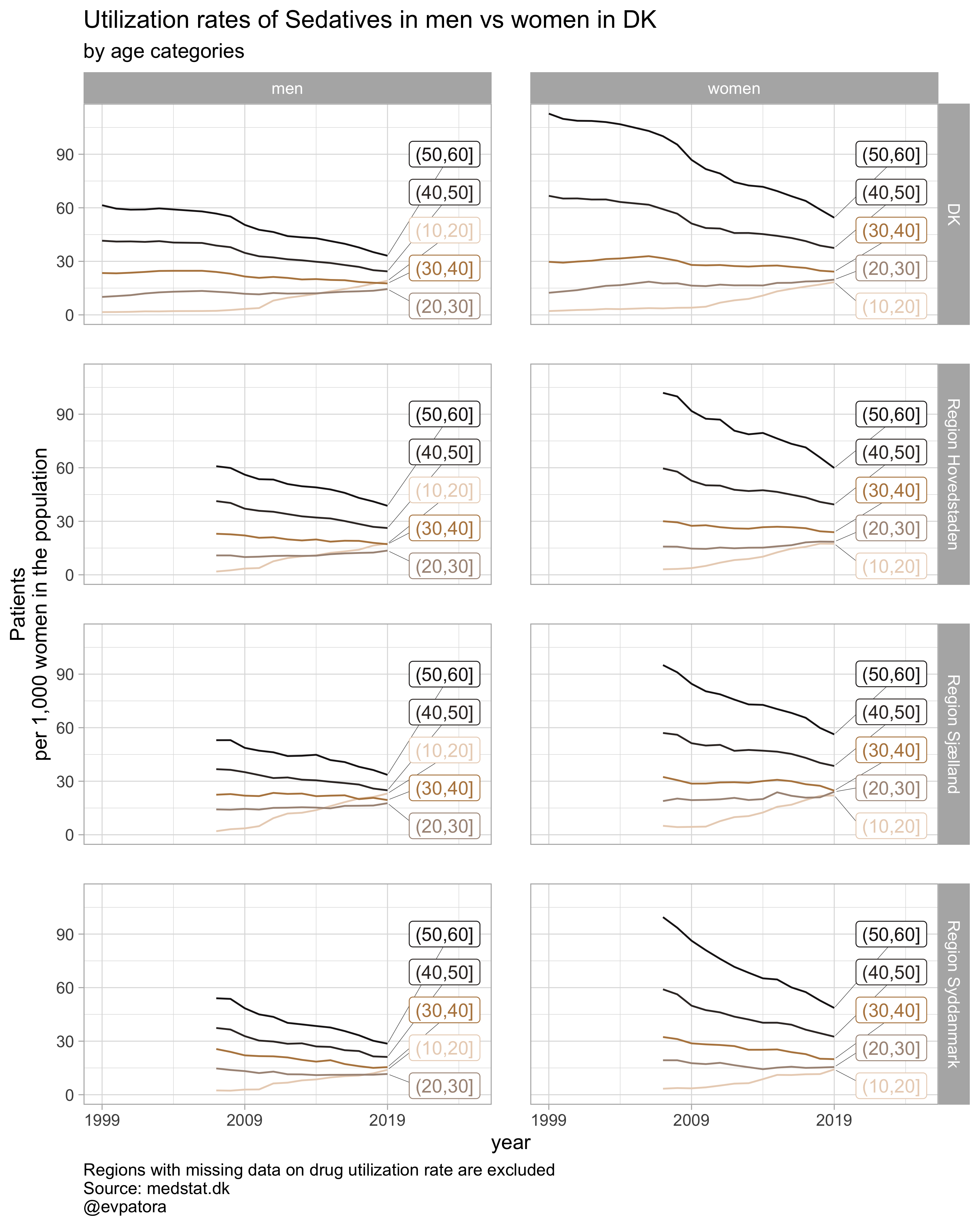
Option 3
# I recode region_var as numeric to simplify my life on the filtering step
# for all regions & for selected age categories, region facets, no age facets
# use different color scheme for each drug with "GrandBudapest1" from {wesanderson} as a default color scheme
plot_utilization <- function(.my_data, drug_regex, atc, age_var, year_var, rate_var, sex_var, title, region_var, region_setting, age_numeric, age_setting, color_setting = "GrandBudapest1", n = 5){

  .my_data %>%
    mutate(
      region_text := case_when(
      {{ region_var }} == "0" ~ "DK",
      {{ region_var }} == "1" ~ "Region Hovedstaden",
      {{ region_var }} == "2" ~ "Region Midtjylland",
      {{ region_var }} == "3" ~ "Region Nordjylland",
      {{ region_var }} == "4" ~ "Region Sjælland",
      {{ region_var }} == "5" ~ "Region Syddanmark",
      T ~ NA_character_
    ),
    {{ region_var }} := as.numeric({{ region_var }})
    ) %>%
    # filter non-missing values on utilization rates
    filter(! is.na({{ rate_var }})) %>%
    filter({{ age_numeric }} %in% age_setting, {{ region_var }} %in% region_setting, str_detect({{ atc }}, drug_regex)) %>%
    # make label for the year 2019
    mutate(label = if_else({{ year_var }} == 2019, as.character({{ age_var }}), NA_character_)) %>%
    ggplot(aes(x = {{ year_var }}, y = {{ rate_var }}, color = {{ age_var }})) +
    geom_path() +
    facet_grid(cols = vars({{ sex_var }}), rows = vars(region_text), scales = "fixed", drop = T) +
    theme_light(base_size = 12) +
    scale_x_continuous(limits = c(1999, 2025), breaks = c(seq(1999, 2019, 10))) +
    expand_limits(y = 0) +
    scale_color_manual(values = wes_palette(name = color_setting, type = "continuous", n = n)) +
    ggrepel::geom_label_repel(aes(label = label), na.rm = TRUE, nudge_x = 4, direction = "y", segment.size = 0.1, segment.colour = "black", show.legend = F) +
    theme(plot.caption = element_text(hjust = 0, size = 10),
          legend.position = "none",
          panel.spacing = unit(0.8, "cm")) +
    labs(y = "Patients\nper 1,000 women in the population", title = paste0(title, " in DK"), subtitle = "by age categories", caption = "Regions with missing data on drug utilization rate are excluded\nSource: medstat.dk\n@evpatora")
}

# 4 drugs for 5 regions by age group
list_regex <- list(regex_antidepress, regex_antipsych, regex_anxiolyt, regex_sedat)
list_drug_name <- list("Antidepressants", "Antipsychotics", "Anxiolytics", "Sedatives")
# compile list of titles from the list of drug names and some text
list_title <- map(list_drug_name, ~paste0("Utilization rates of ", .x, " in men vs women"))
# list of colors to iterate along; each color will correspond to the drug class
list_color <- list("GrandBudapest1", "GrandBudapest2", "IsleofDogs1", "IsleofDogs2")

# iteration
list_plots <- pmap(.l = list(list_regex, list_title, list_color),
                   .f = ~plot_utilization(.my_data = data, atc = ATC, drug_regex = ..1, age_var = age_cat,
                                          year_var = year, rate_var = patients_per_1000_inhabitants, sex_var = gender_text,
                                          title = ..2, region_var = region, region_setting = 0:5, age_numeric = age,
                                          age_setting = 10:60, color_setting = ..3))

# see some results
list_plots
## [[1]]
##
## [[2]]
##
## [[3]]
##
## [[4]]
# save all plots with one line: each saved plot has the name of the plotted characteristics
walk2(.x = list_plots, .y = list_title, ~ggsave(filename = paste0(Sys.Date(), "-", .y, ".pdf"),
                                                plot = .x, path = getwd(), device = cairo_pdf,
                                                width = 297, height = 210, units = "mm"))
Take home messages
- Some copy-pasting is hard to avoid
- Developing understanding of your data will also improve your understanding of how to create more flexible custom functions
- When optimized, visualization leaves more space to concentrate on interpretation of data
Cheers! ✌️