TidyTuesday Spice Girls Data

Data

I use data by Jacquie Tran available here. Let’s go ✌

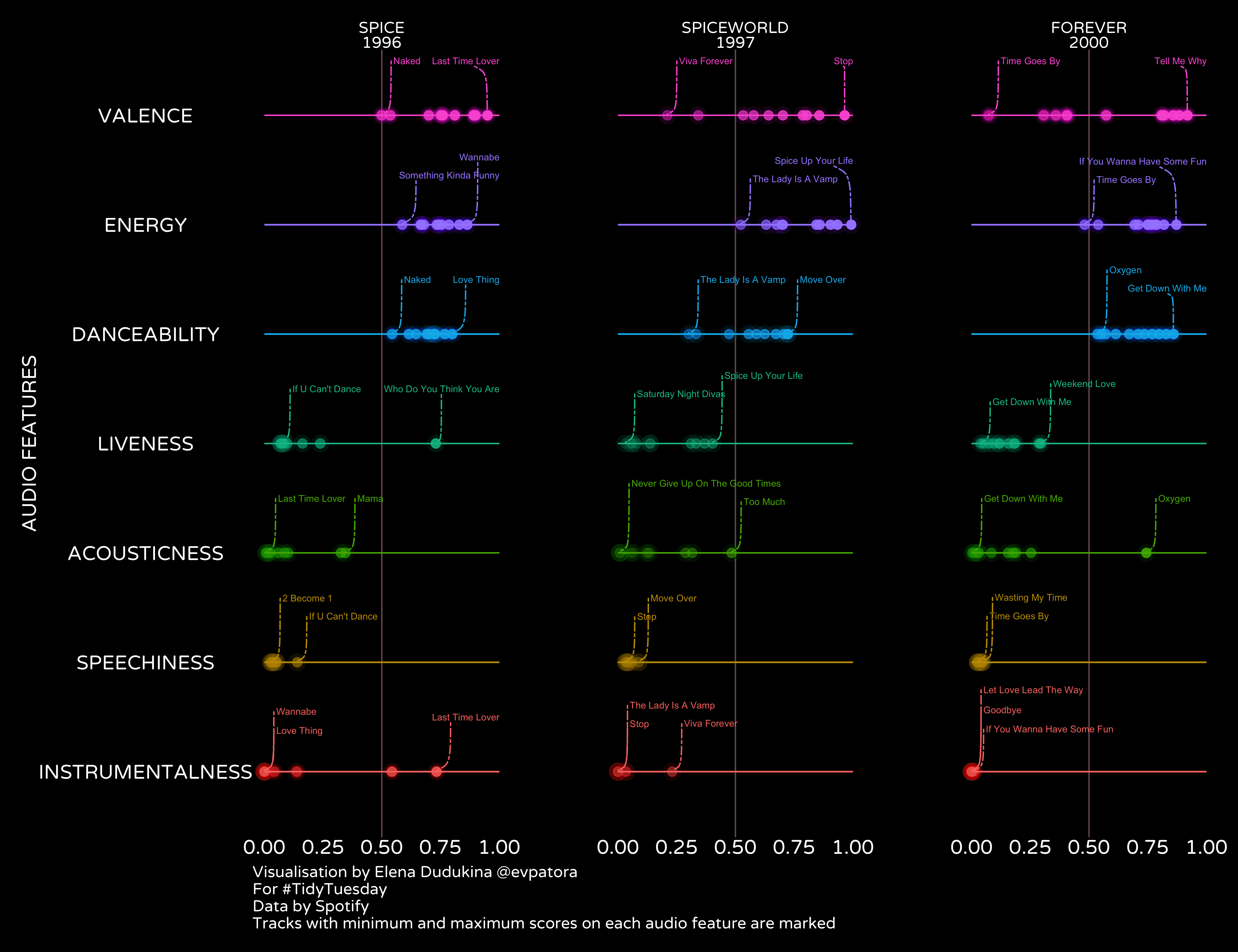
I chose to plot the audio features of Spice Girls tracks: danceability, energy, speechiness, acousticness, valence, liveness, and instrumentalness. Each of these are measures from 0.0 to 1.0, which represents a certain perceptual feature.

library(tidyverse)
library(magrittr)
library(ggblur)

spice_tracks <- readr::read_csv("https://github.com/jacquietran/spice_girls_data/raw/main/data/studio_album_tracks.csv")

## Rows: 31 Columns: 25

## ── Column specification ────────────────────────────────────────────────────────
## Delimiter: ","
## chr   (9): artist_name, artist_id, album_id, track_id, track_name, album_nam...
## dbl  (15): album_release_year, danceability, energy, key, loudness, mode, sp...
## date  (1): album_release_date

## 
## ℹ Use `spec()` to retrieve the full column specification for this data.
## ℹ Specify the column types or set `show_col_types = FALSE` to quiet this message.

spice_tracks %>% names(.)

##  [1] "artist_name"        "artist_id"          "album_id"          
##  [4] "album_release_date" "album_release_year" "danceability"      
##  [7] "energy"             "key"                "loudness"          
## [10] "mode"               "speechiness"        "acousticness"      
## [13] "instrumentalness"   "liveness"           "valence"           
## [16] "tempo"              "track_id"           "time_signature"    
## [19] "duration_ms"        "track_name"         "track_number"      
## [22] "album_name"         "key_name"           "mode_name"         
## [25] "key_mode"

Plot

spice_tracks %<>% 
  pivot_longer(cols = c(danceability, energy, acousticness, speechiness, instrumentalness, liveness, valence), names_to = "AUDIO FEATURES", values_to = "score")

spice_plot <- spice_tracks %>% 
  mutate(
    `AUDIO FEATURES` = str_to_upper(`AUDIO FEATURES`),
    `AUDIO FEATURES` = forcats::fct_reorder(`AUDIO FEATURES`, score),
    album_name = str_to_upper(album_name),
    album_name = factor(album_name, levels = c("SPICE", "SPICEWORLD", "FOREVER")),
  ) %>% 
  group_by(album_name,`AUDIO FEATURES`) %>% 
  mutate(
    label = case_when(
      score == min(score) ~ track_name,
      score == max(score) ~ track_name,
      T ~ NA_character_
    )
  ) %>% 
  ungroup() %>% 
  group_by(album_name,`AUDIO FEATURES`, score) %>% 
  filter(row_number() == 1 | row_number() == n()) %>% 
  ungroup() %>% 
  arrange(album_name) %>% 
  ggplot(aes(y = `AUDIO FEATURES`, x = score, group = album_name, color = `AUDIO FEATURES`, fill = `AUDIO FEATURES`)) + 
  scale_x_continuous(breaks = seq(0, 1, 0.25)) +
  geom_vline(xintercept = 0.5, color = "pink", alpha = 0.4) +
  facet_grid(cols = vars(album_name, album_release_year)) +
  theme_void(base_family = "Varela Round", base_size = 15) +
  # sparkly point
  geom_point_blur(blur_steps = 150, size = 3, aes(alpha = score + 0.1)) +
  ggforce::geom_link(aes(y = `AUDIO FEATURES`, yend = `AUDIO FEATURES`, x = 0, xend = 1, color = `AUDIO FEATURES`)) +
  theme(
    plot.background = element_rect(fill = "black"),
    text = element_text(color = "white"),
    axis.title.y = element_text(color = "white", angle = 90),
    axis.text.y = element_text(color = "white"),
    legend.position = "none",
    legend.box.margin = margin(2, 2, 2, 2),
    axis.text.x = element_text(color = "white"),
    panel.spacing = unit(5, "lines"),
    plot.margin = margin(15, 15, 15, 15),
    plot.caption = element_text(hjust = 0)
  ) +
  ggrepel::geom_text_repel(mapping = aes(label = label), segment.curvature = -0.3, box.padding = 0.3, nudge_y = 0.5, nudge_x = 0.075, segment.linetype = 6, direction = "y", hjust = "left", size = 2.5) +
  labs(caption = "Visualisation by Elena Dudukina @evpatora\nFor #TidyTuesday\nData by Spotify\nTracks with minimum and maximum scores on each audio feature are marked")
  
spice_plot

## Warning: Removed 166 rows containing missing values (geom_text_repel).

ggsave(spice_plot, filename = "spice.jpeg", dpi = 400, units = "cm", width = 29.7, height = 20, path = path)

## Warning: Removed 166 rows containing missing values (geom_text_repel).