TidyTuesday 2022: week 1

Data

I’m going to use the data I’m intimately familiar with: medication utilization in Denmark. I will visualize antidepressants use patterns. I’ll use palettes from my {hermitage} package.

My favourite palettes so far are madonna_litta and hermitage_1.

library(tidyverse)
library(magrittr)
library(hermitage)

Plots

col <- hermitage_palette("parsons_2")
set.seed(876555)
values <- sample(x = col, size = 3)

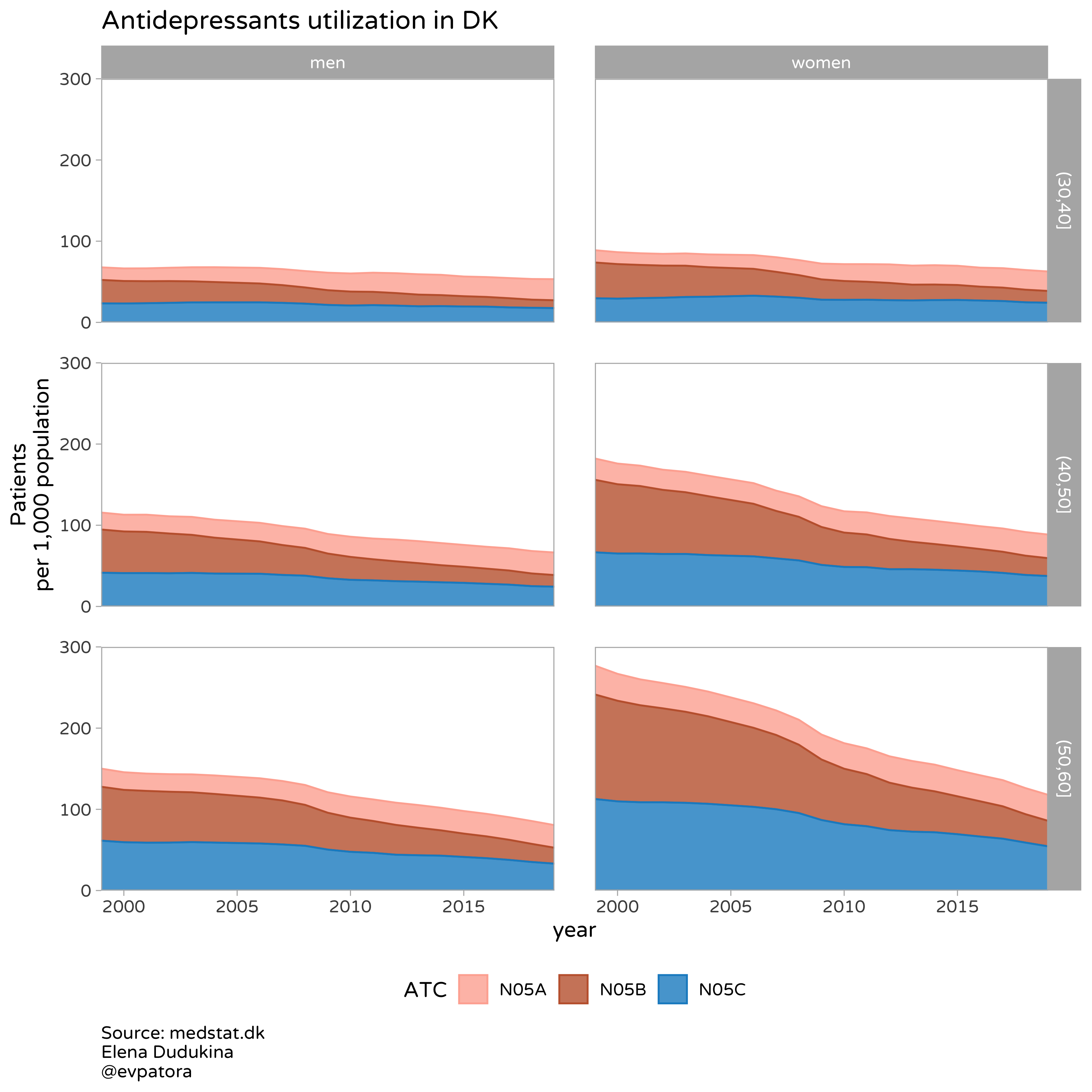
plot <- atc_2 %>%
  ggplot(aes(x = year, y = patients_per_1000_inhabitants, color = ATC, fill = ATC)) +
  geom_area(alpha = 0.8, outline.type = NULL) +
  facet_grid(cols = vars(gender_text), rows = vars(age_cat), scales = "fixed", drop = T) +
  theme_light(base_size = 12, base_family = "Varela Round") +
  scale_color_manual(values = values) +
  scale_fill_manual(values = values) +
  scale_x_continuous(expand = c(0,0)) +
  scale_y_continuous(expand = c(0,0), limits = c(0, 300)) +
  theme(plot.caption = element_text(hjust = 0, size = 10),
        legend.position = "bottom",
        panel.spacing = unit(0.8, "cm"),
        panel.grid = element_blank()) +
  labs(y = "Patients\nper 1,000 population",
       title = paste0("Antidepressants utilization in DK"),
       caption = "Source: medstat.dk\nElena Dudukina\n@evpatora")

# note that area plot is a stacked graph (do not read as geom_path plot)
plot

ggsave(plot, filename = "plot_1.jpeg", dpi = 400, units = "cm", width = 29.7, height = 20, path = path)

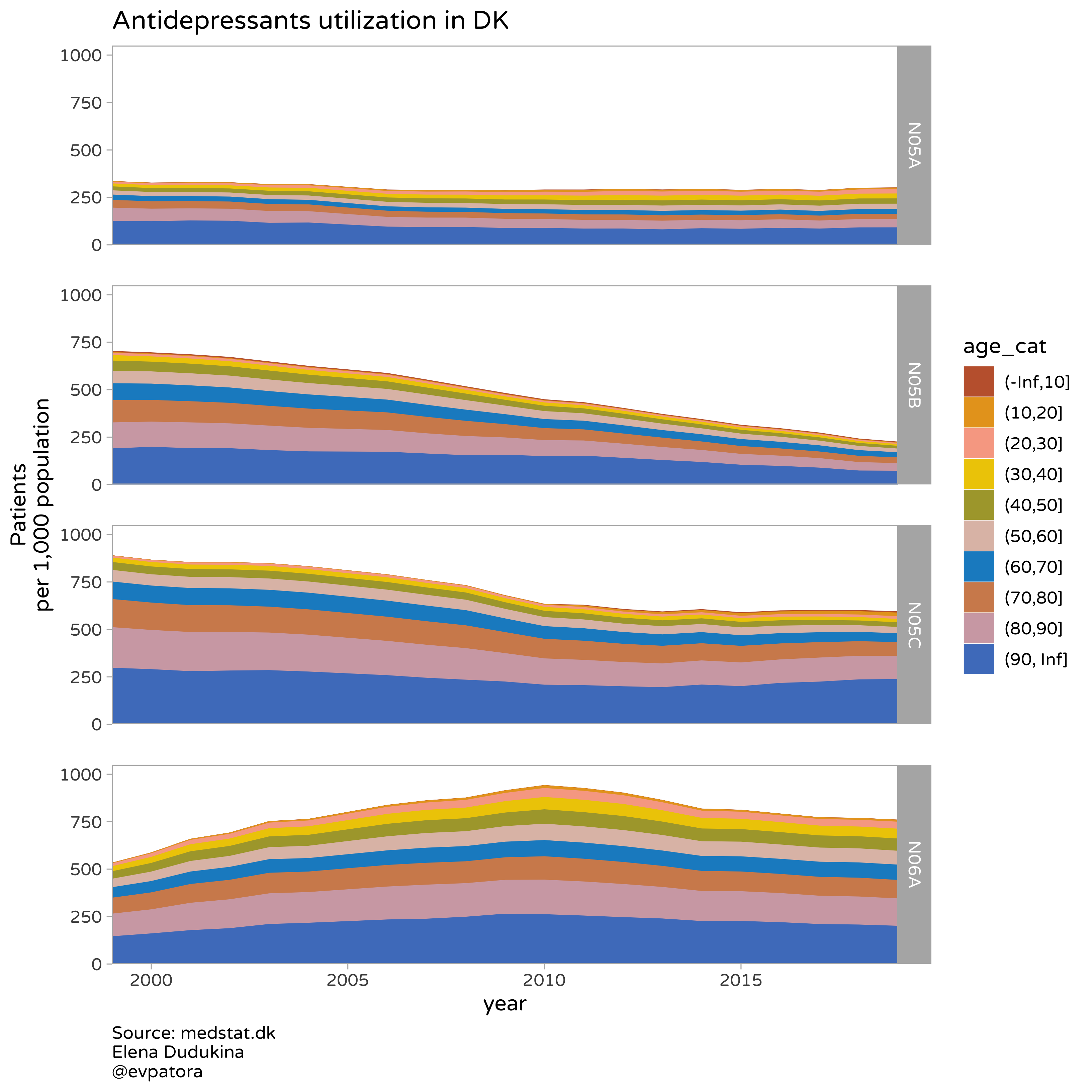
col <- hermitage_palette("parsons_2")
plot <- atc_3 %>%
  ggplot(aes(x = year, y = patients_per_1000_inhabitants, color = age_cat, fill = age_cat)) +
  geom_area(outline.type = NULL) +
  facet_grid(rows = vars(ATC), scales = "fixed", drop = T) +
  theme_light(base_size = 12, base_family = "Varela Round") +
  scale_x_continuous(expand = c(0,0)) +
  scale_y_continuous(expand = c(0,0), limits = c(0, 1050)) +
  scale_color_manual(values = col) +
  scale_fill_manual(values = col) +
  theme(plot.caption = element_text(hjust = 0, size = 10),
        legend.position = "right",
        panel.spacing = unit(0.8, "cm"),
        panel.grid = element_blank()) +
  labs(y = "Patients\nper 1,000 population", title = paste0("Antidepressants utilization in DK"),
       caption = "Source: medstat.dk\nElena Dudukina\n@evpatora")

# note that area plot is a stacked graph (do not read as geom_path plot)
plot

ggsave(plot, filename = "plot_2.jpeg", dpi = 400, units = "cm", width = 29.7, height = 20, path = path)

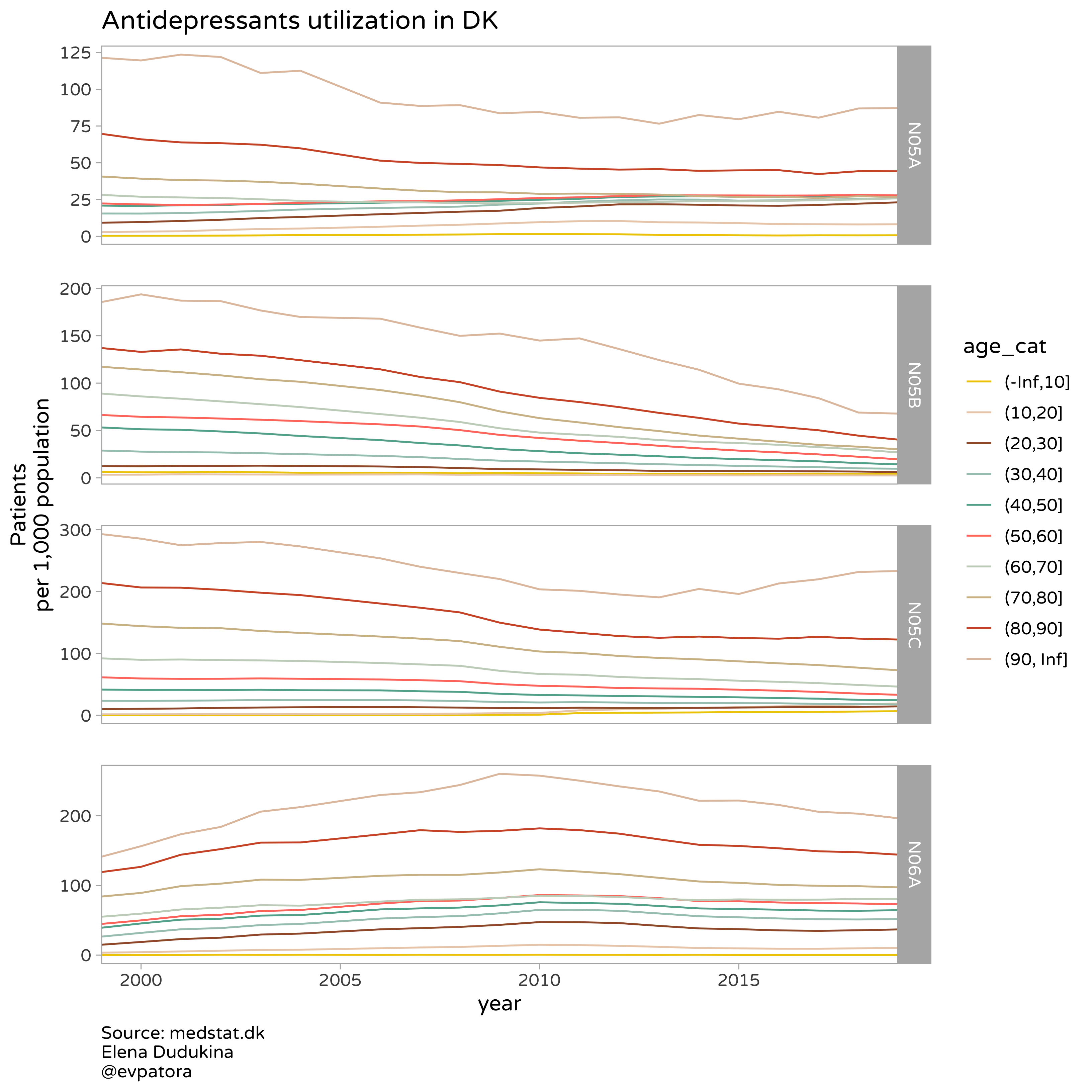
col <- hermitage_palette("parsons_2")
set.seed(87655567)
values <- sample(x = col, size = 10, replace = F)

plot <- atc_3 %>%
  ggplot(aes(x = year, y = patients_per_1000_inhabitants, color = age_cat, fill = age_cat)) +
  geom_path() +
  facet_grid(rows = vars(ATC), scales = "free", drop = T) +
  theme_light(base_size = 12, base_family = "Varela Round") +
  scale_x_continuous(expand = c(0,0)) +
  scale_color_manual(values = values) +
  scale_fill_manual(values = values) +
  theme(plot.caption = element_text(hjust = 0, size = 10),
        legend.position = "right",
        panel.spacing = unit(0.8, "cm"),
        panel.grid = element_blank()) +
  labs(y = "Patients\nper 1,000 population", title = paste0("Antidepressants utilization in DK"),
       caption = "Source: medstat.dk\nElena Dudukina\n@evpatora")

plot

ggsave(plot, filename = "plot_3.jpeg", dpi = 400, units = "cm", width = 29.7, height = 20, path = path)

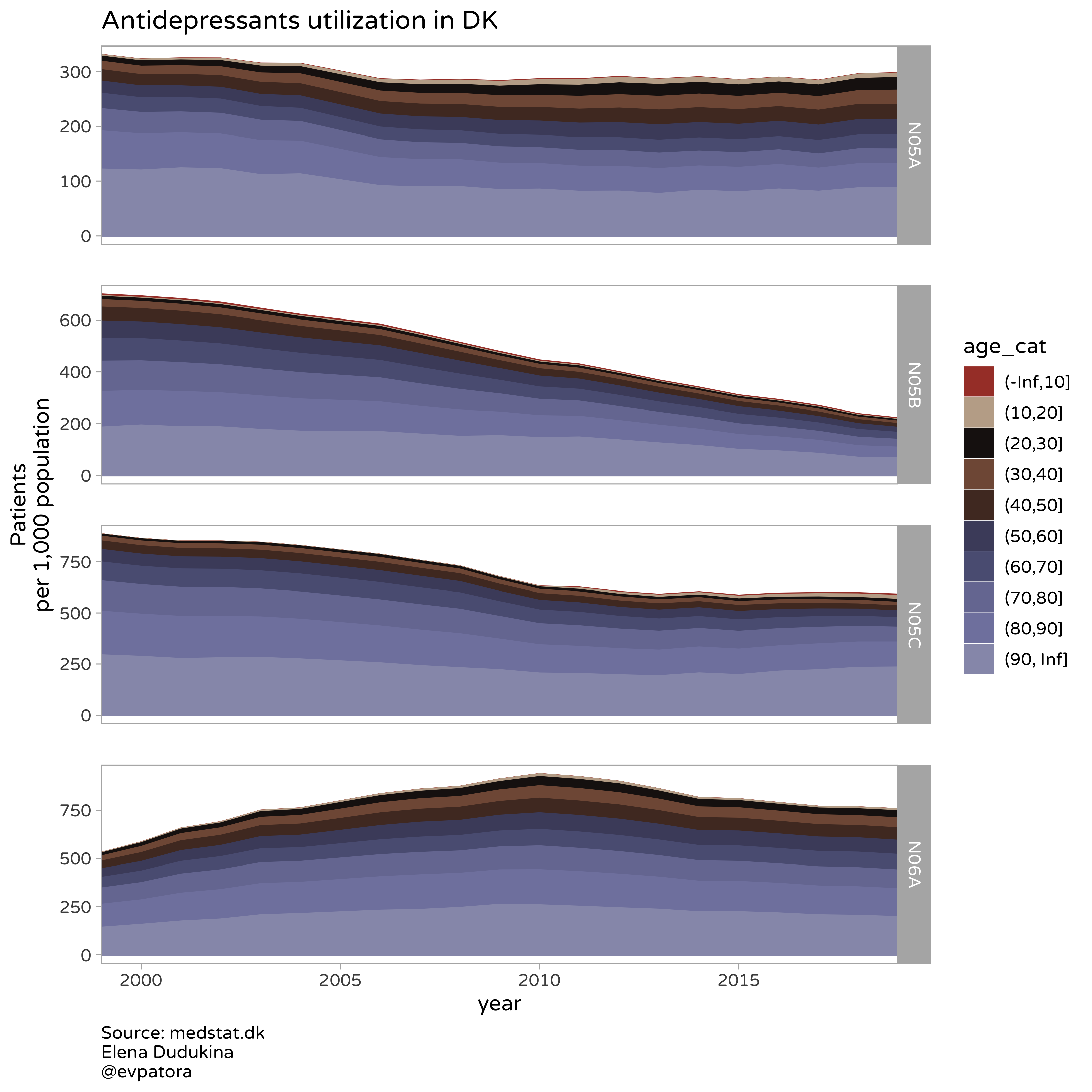
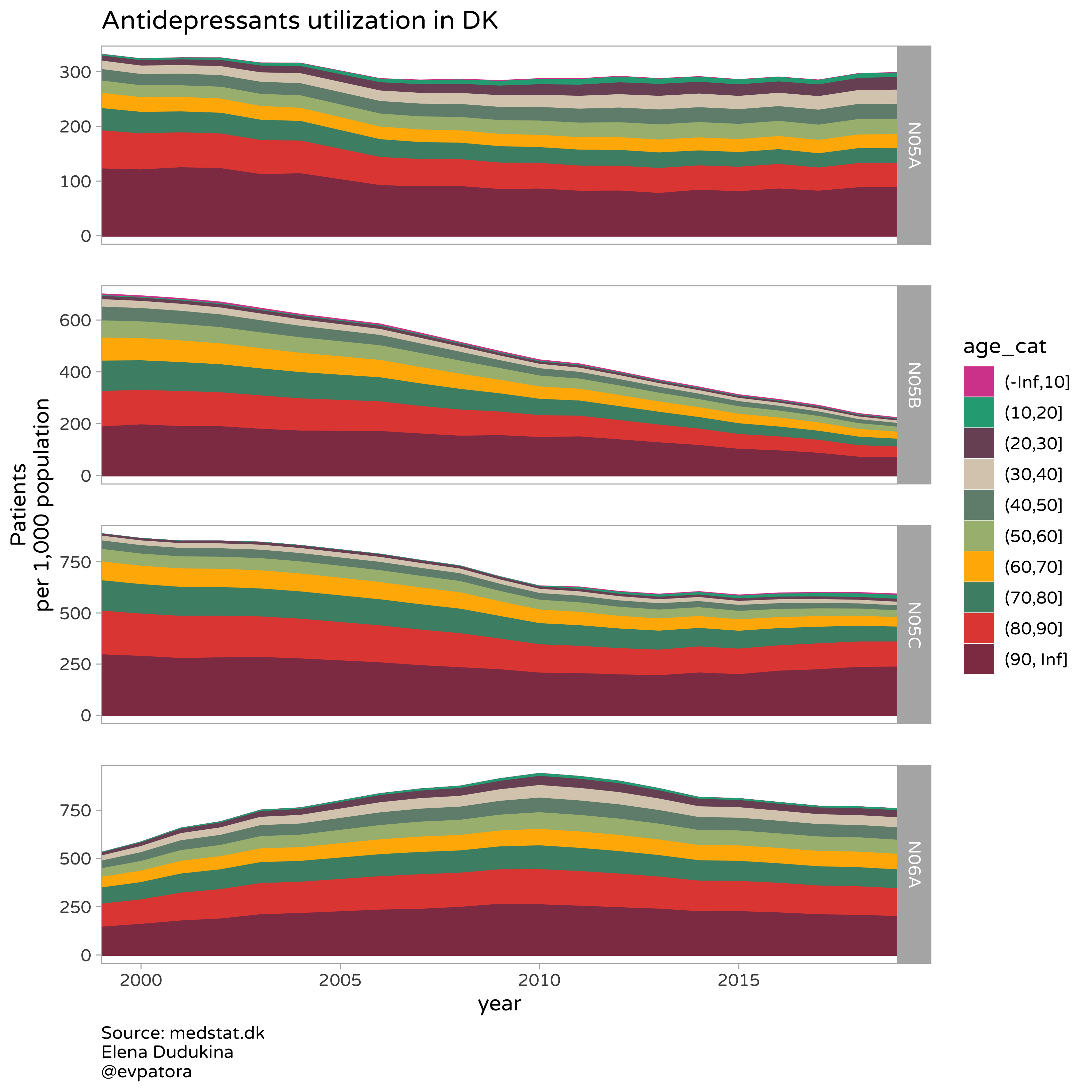
col <- hermitage_palette("madonna_litta")
plot <- atc_3 %>%
  ggplot(aes(x = year, y = patients_per_1000_inhabitants, color = age_cat, fill = age_cat)) +
  geom_area(outline.type = NULL) +
  facet_grid(rows = vars(ATC), scales = "free", drop = T) +
  theme_light(base_size = 12, base_family = "Varela Round") +
  expand_limits(y = 0) +
  scale_x_continuous(expand = c(0,0)) +
  scale_color_manual(values = col) +
  scale_fill_manual(values = col) +
  theme(plot.caption = element_text(hjust = 0, size = 10),
        legend.position = "right",
        panel.spacing = unit(0.8, "cm"),
        panel.grid = element_blank()) +
  labs(y = "Patients\nper 1,000 population",
       title = paste0("Antidepressants utilization in DK"),
       caption = "Source: medstat.dk\nElena Dudukina\n@evpatora")

plot

ggsave(plot, filename = "plot_4.jpeg", dpi = 400, units = "cm", width = 29.7, height = 20, path = path)

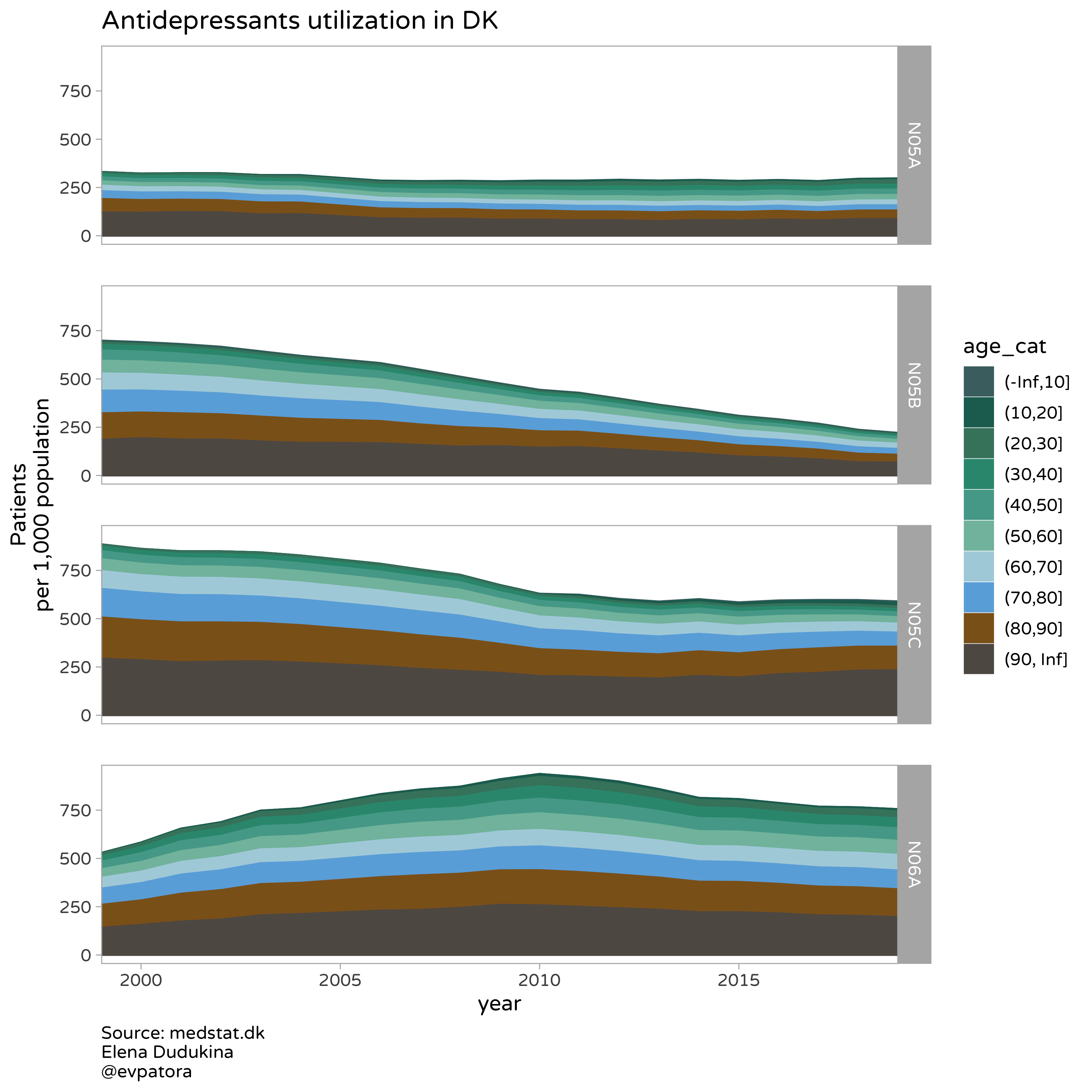
col <- hermitage_palette("hermitage_1")
plot <- atc_3 %>%
  ggplot(aes(x = year, y = patients_per_1000_inhabitants, color = age_cat, fill = age_cat)) +
  geom_area(outline.type = NULL) +
  facet_grid(rows = vars(ATC), scales = "fixed", drop = T) +
  theme_light(base_size = 12, base_family = "Varela Round") +
  expand_limits(y = 0) +
  scale_x_continuous(expand = c(0,0)) +
  scale_color_manual(values = col) +
  scale_fill_manual(values = col) +
  theme(plot.caption = element_text(hjust = 0, size = 10),
        legend.position = "right",
        panel.spacing = unit(0.8, "cm"),
        panel.grid = element_blank()) +
  labs(y = "Patients\nper 1,000 population",
       title = paste0("Antidepressants utilization in DK"),
       caption = "Source: medstat.dk\nElena Dudukina\n@evpatora")
# note that area plot is a stacked graph (do not read as geom_path plot)
plot

ggsave(plot, filename = "plot_5.jpeg", dpi = 400, units = "cm", width = 29.7, height = 20, path = path)

col <- hermitage_palette("parsons_2")
set.seed(55276511)
values <- sample(x = col, size = 10, replace = FALSE)

plot <- atc_3 %>%
  ggplot(aes(x = year, y = patients_per_1000_inhabitants, color = age_cat, fill = age_cat)) +
  geom_area(outline.type = NULL) +
  facet_grid(rows = vars(ATC), scales = "free", drop = T) +
  theme_light(base_size = 12, base_family = "Varela Round") +
  expand_limits(y = 0) +
  scale_x_continuous(expand = c(0,0)) +
  scale_color_manual(values = values) +
  scale_fill_manual(values = values) +
  theme(plot.caption = element_text(hjust = 0, size = 10),
        legend.position = "right",
        panel.spacing = unit(0.8, "cm"),
        panel.grid = element_blank()) +
  labs(y = "Patients\nper 1,000 population",
       title = paste0("Antidepressants utilization in DK"),
       caption = "Source: medstat.dk\nElena Dudukina\n@evpatora")

plot

ggsave(plot, filename = "plot_6.jpeg", dpi = 400, units = "cm", width = 29.7, height = 20, path = path)