Kaggle ML survey 2021
I am a doctoral student. I often wonder what my future holds in this brave and largely liberated according to some world. In EU, although 48% of doctoral graduates were women according to She Figures 2021, only 34% of researchers are women and only 24% of heads of higher education institutions are women. Even worse the situation is with equality in inventorship, where only 10% are women. This is women to men ratio of 0.12%.
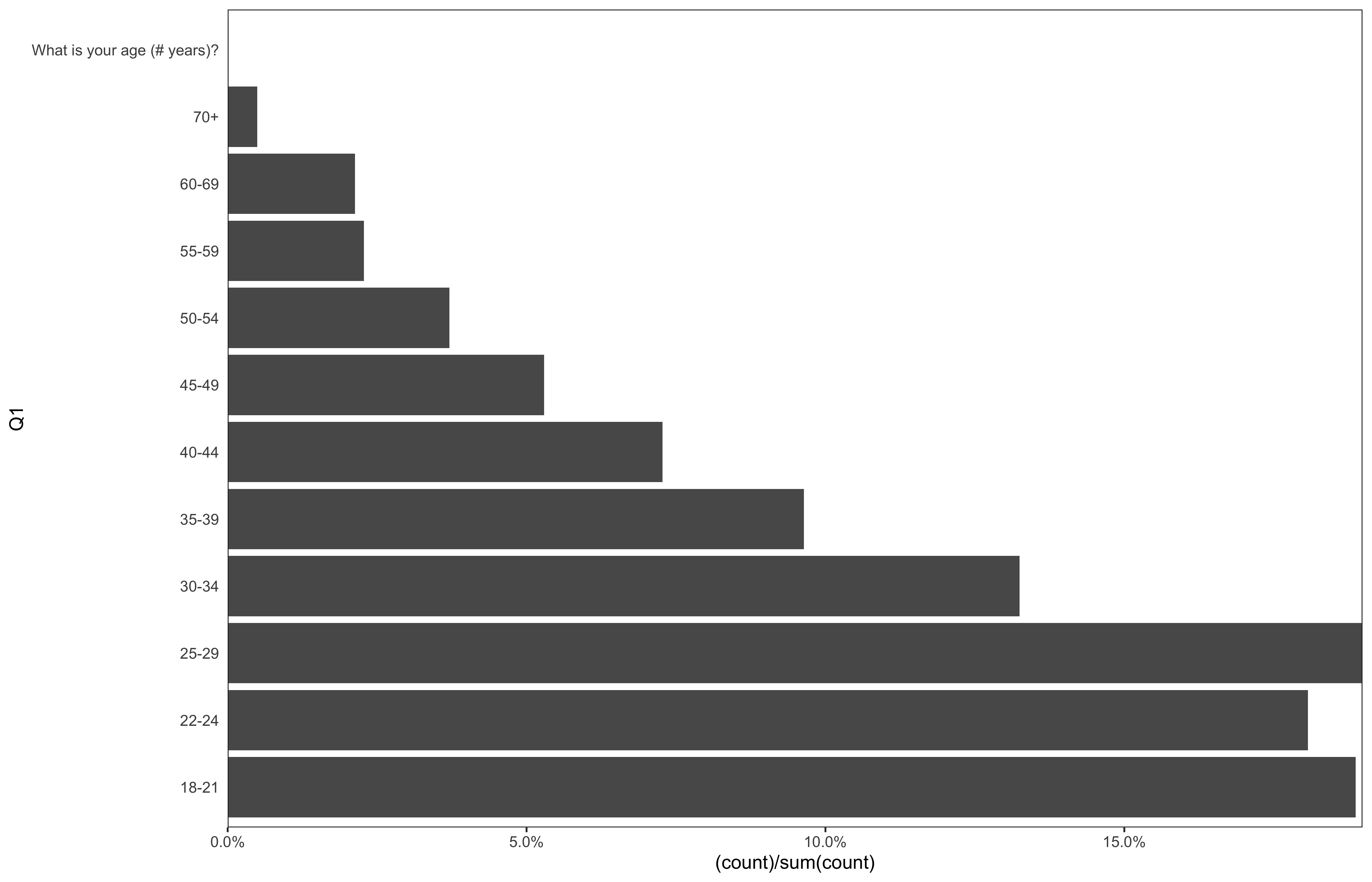
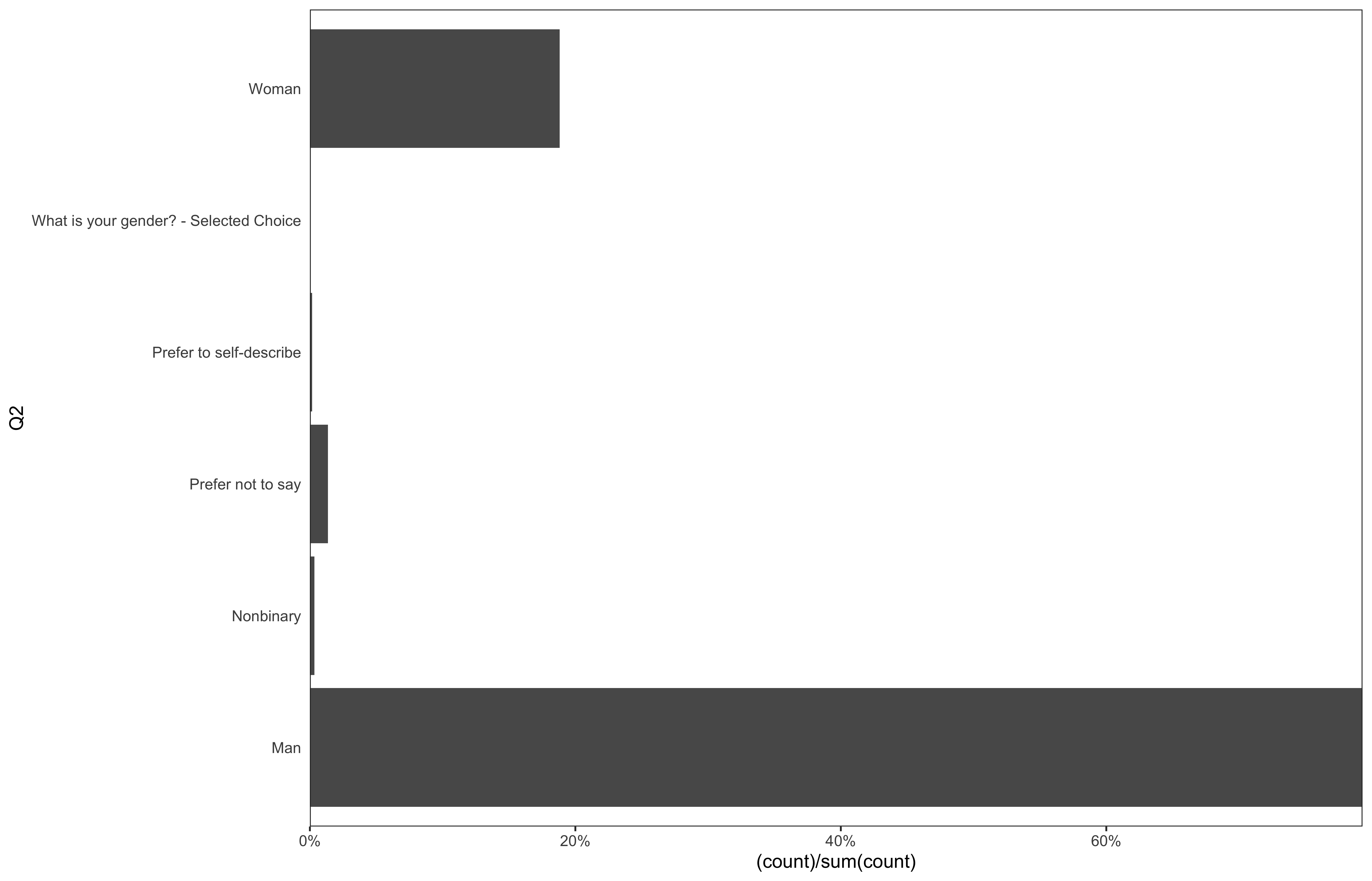
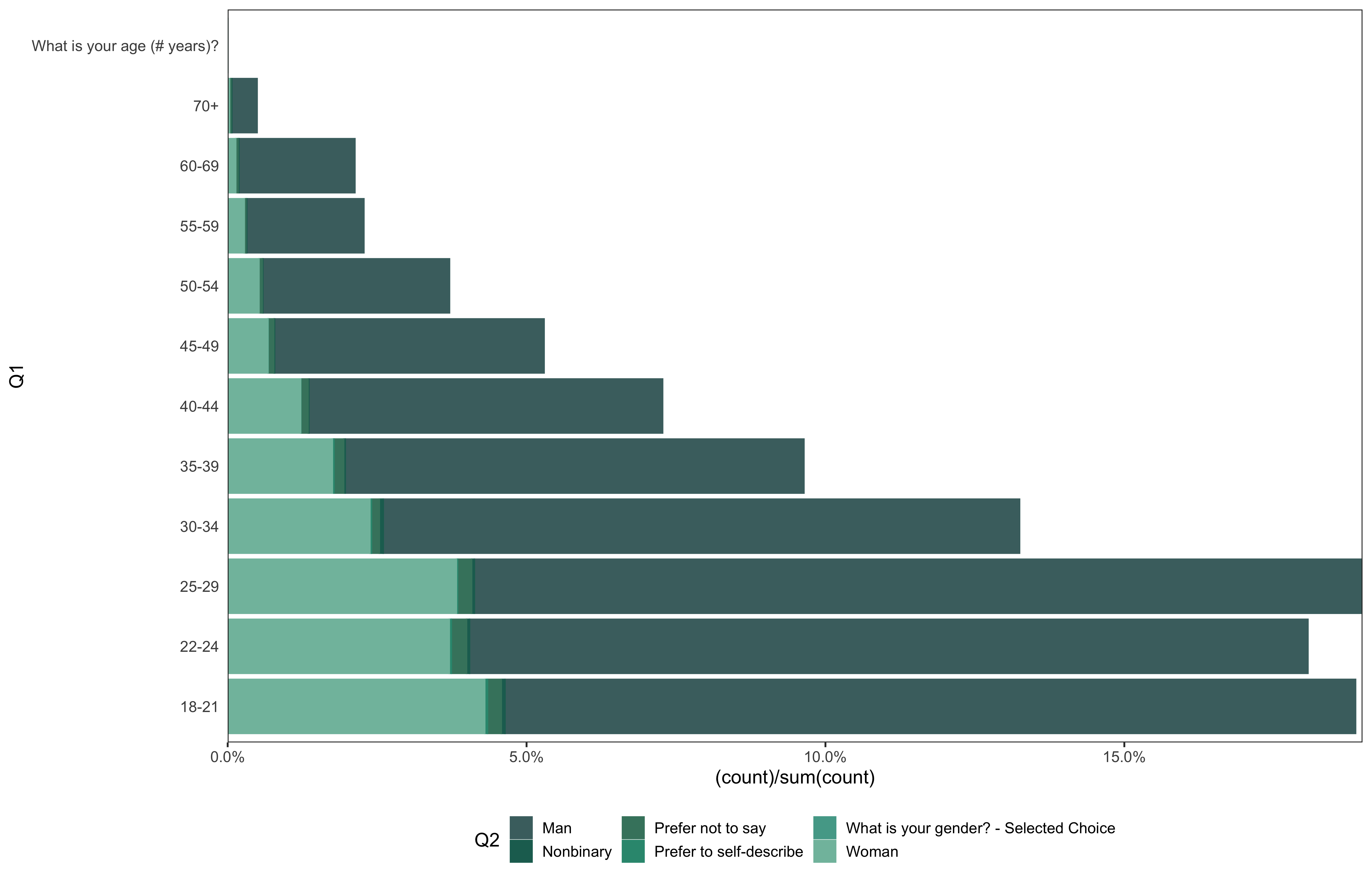
I was wondering for a while now, what is the gender distribution among Kaggle participants in recent years. I took 2021 data as a study case and looked at the gender distribution among respondents of several survey questions.
Data
The data I use are available here.
library(tidyverse)
library(magrittr)
library(hermitage)
data <- read_csv(file = paste0(path, "kaggle_survey_2021_responses.csv"))
## Rows: 25974 Columns: 369
## ── Column specification ────────────────────────────────────────────────────────
## Delimiter: ","
## chr (369): Time from Start to Finish (seconds), Q1, Q2, Q3, Q4, Q5, Q6, Q7_P...
##
## ℹ Use `spec()` to retrieve the full column specification for this data.
## ℹ Specify the column types or set `show_col_types = FALSE` to quiet this message.
Exploratory plots
data %>%
  ggplot(aes(x = Q1)) +
  geom_bar(aes(y = (..count..)/sum(..count..))) +
  theme_bw(base_size = 14) +
  scale_y_continuous(expand = c(0, 0), labels = scales::percent) +
  theme(plot.caption = element_text(hjust = 0, size = 10),
        legend.position = "bottom",
        panel.spacing = unit(0.8, "cm"),
        panel.grid = element_blank(),
        axis.ticks.y = element_blank()) +
  coord_flip()
data %>%
  ggplot(aes(x = Q2)) +
  geom_bar(aes(y = (..count..)/sum(..count..))) +
  theme_bw(base_size = 14) +
  scale_y_continuous(expand = c(0, 0), labels = scales::percent) +
  theme(plot.caption = element_text(hjust = 0, size = 10),
        legend.position = "bottom",
        panel.spacing = unit(0.8, "cm"),
        panel.grid = element_blank(),
        axis.ticks.y = element_blank()) +
  coord_flip()
data %>%
  ggplot(aes(x = Q1, group = Q2, color = Q2, fill = Q2)) +
  geom_bar(aes(y = (..count..)/sum(..count..)), position = position_stack()) +
  theme_bw(base_size = 14) +
  scale_y_continuous(expand = c(0, 0), labels = scales::percent) +
  theme(plot.caption = element_text(hjust = 0, size = 10),
        legend.position = "bottom",
        panel.spacing = unit(0.8, "cm"),
        panel.grid = element_blank(),
        axis.ticks.y = element_blank()) +
  coord_flip() +
  scale_color_manual(values = hermitage::hermitage_palette(name = "hermitage_1")) +
  scale_fill_manual(values = hermitage::hermitage_palette(name = "hermitage_1"))
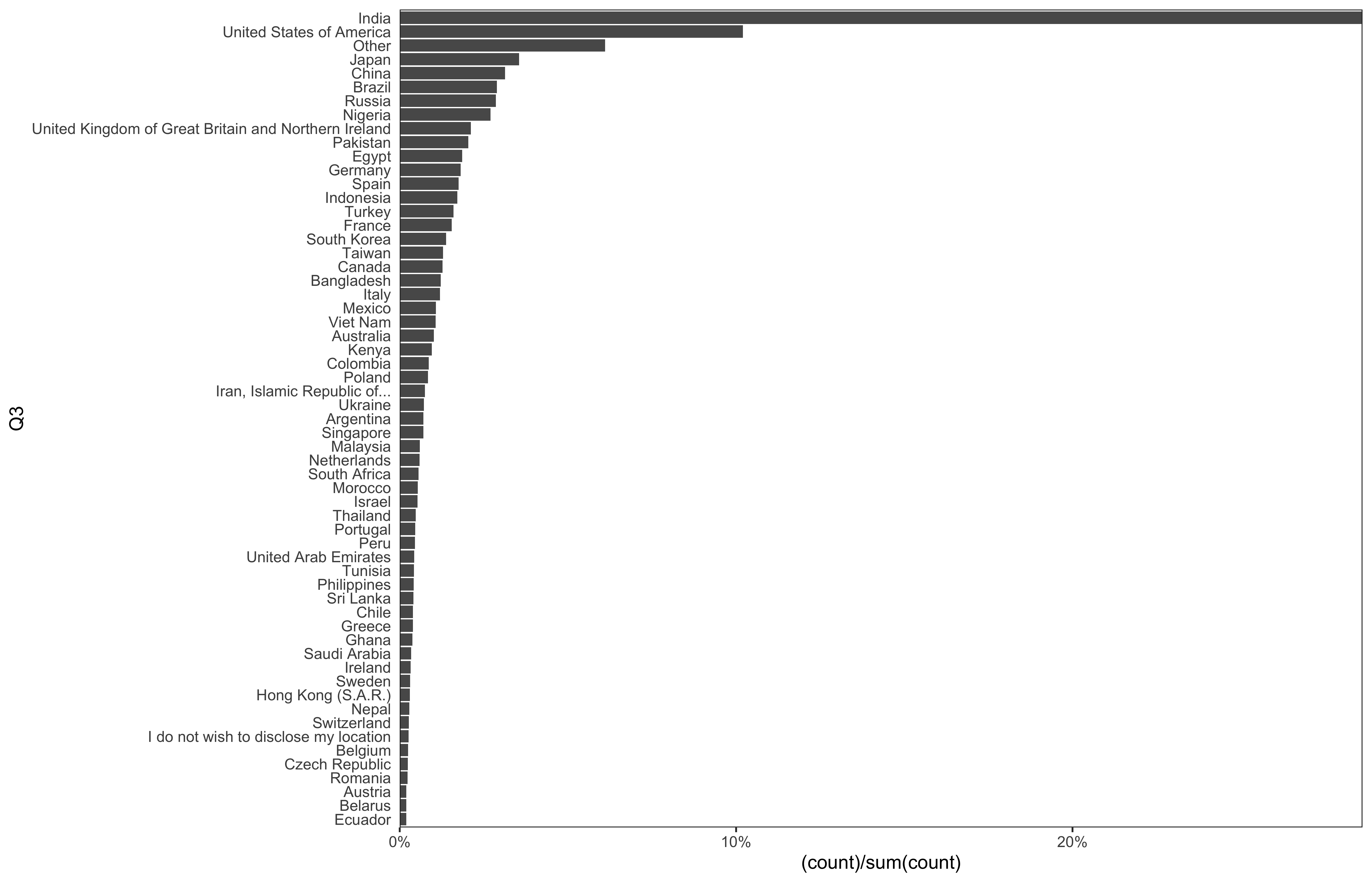
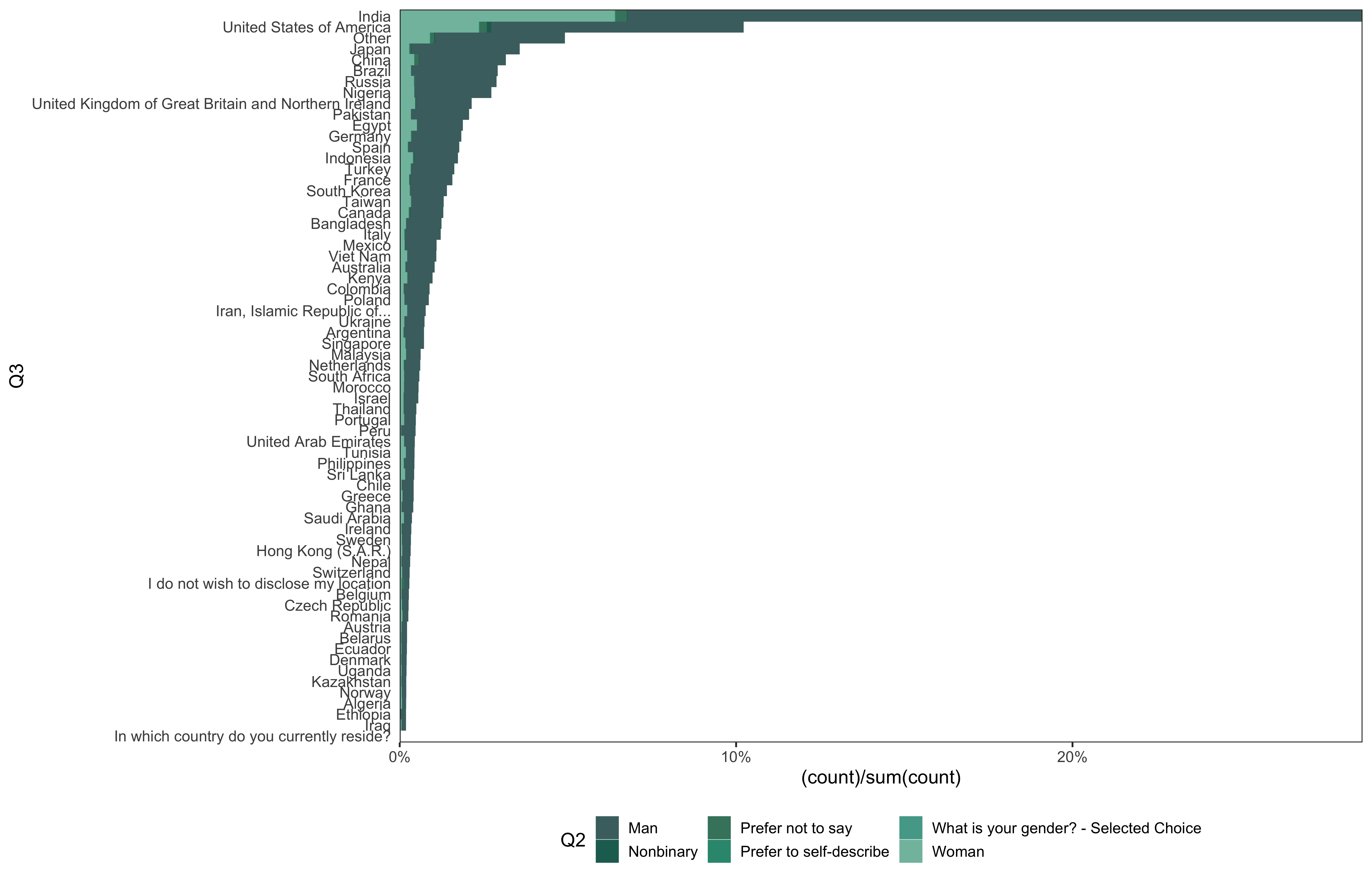
data %>%
  mutate(
    Q3 = fct_lump_min(Q3, min = 50),
    Q3 = factor(Q3),
    Q3 = fct_rev(fct_infreq(Q3))
  ) %>%
  ggplot(aes(x = Q3)) +
  geom_bar(aes(y = (..count..)/sum(..count..))) +
  theme_bw(base_size = 14) +
  scale_y_continuous(expand = c(0, 0), labels = scales::percent) +
  theme(plot.caption = element_text(hjust = 0, size = 10),
        legend.position = "bottom",
        panel.spacing = unit(0.8, "cm"),
        panel.grid = element_blank(),
        axis.ticks.y = element_blank()) +
  coord_flip()
go <- function(.data, variable, group = Q2){
  .data %>%
  mutate(
    {{ variable }} := factor({{ variable }}),
    {{ variable }} := fct_rev(fct_infreq({{ variable }}))
  ) %>%
  ggplot(aes(x = {{ variable }}, group = {{ group }}, fill = {{ group }}, color = {{ group }})) +
  geom_bar(aes(y = (..count..)/sum(..count..))) +
  theme_bw(base_size = 14) +
  scale_y_continuous(expand = c(0, 0), labels = scales::percent) +
  theme(plot.caption = element_text(hjust = 0, size = 10),
        legend.position = "bottom",
        panel.spacing = unit(0.8, "cm"),
        panel.grid = element_blank(),
        axis.ticks.y = element_blank()) +
  coord_flip() +
  scale_color_manual(values = hermitage::hermitage_palette(name = "hermitage_1")) +
  scale_fill_manual(values = hermitage::hermitage_palette(name = "hermitage_1"))
}
data %>%
  go(Q3)
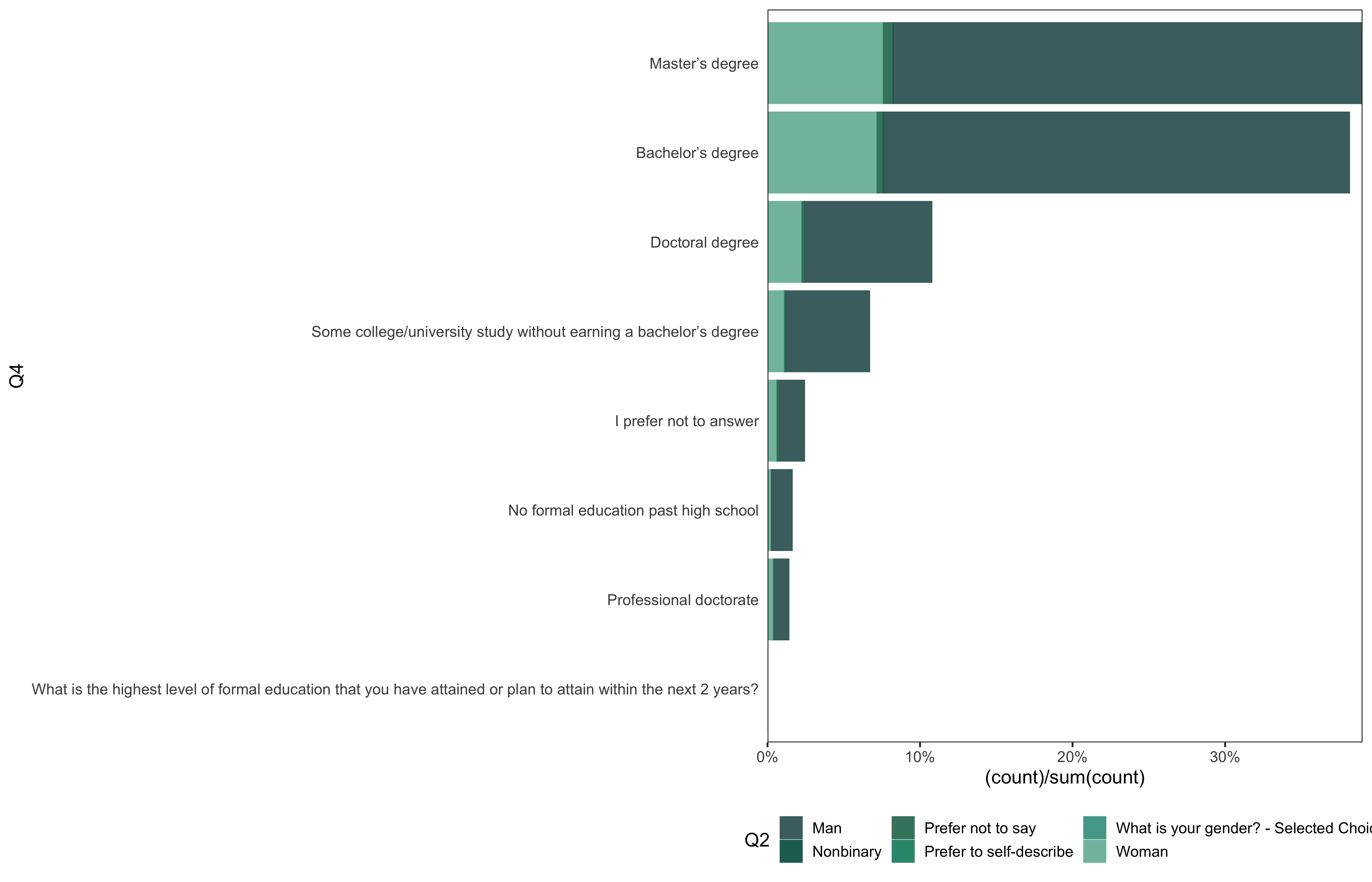
data %>%
  go(Q4)
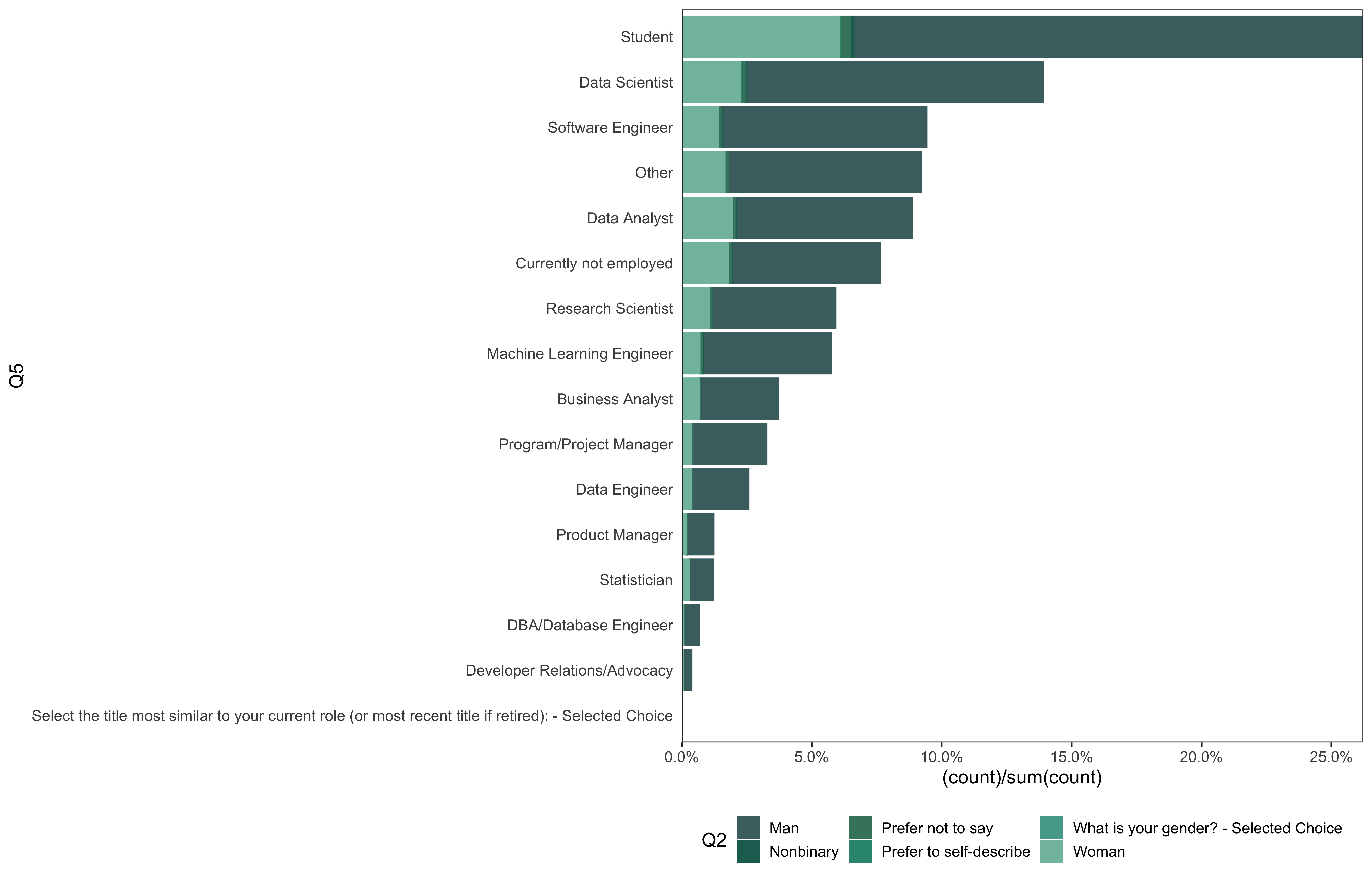
data %>%
  go(Q5)
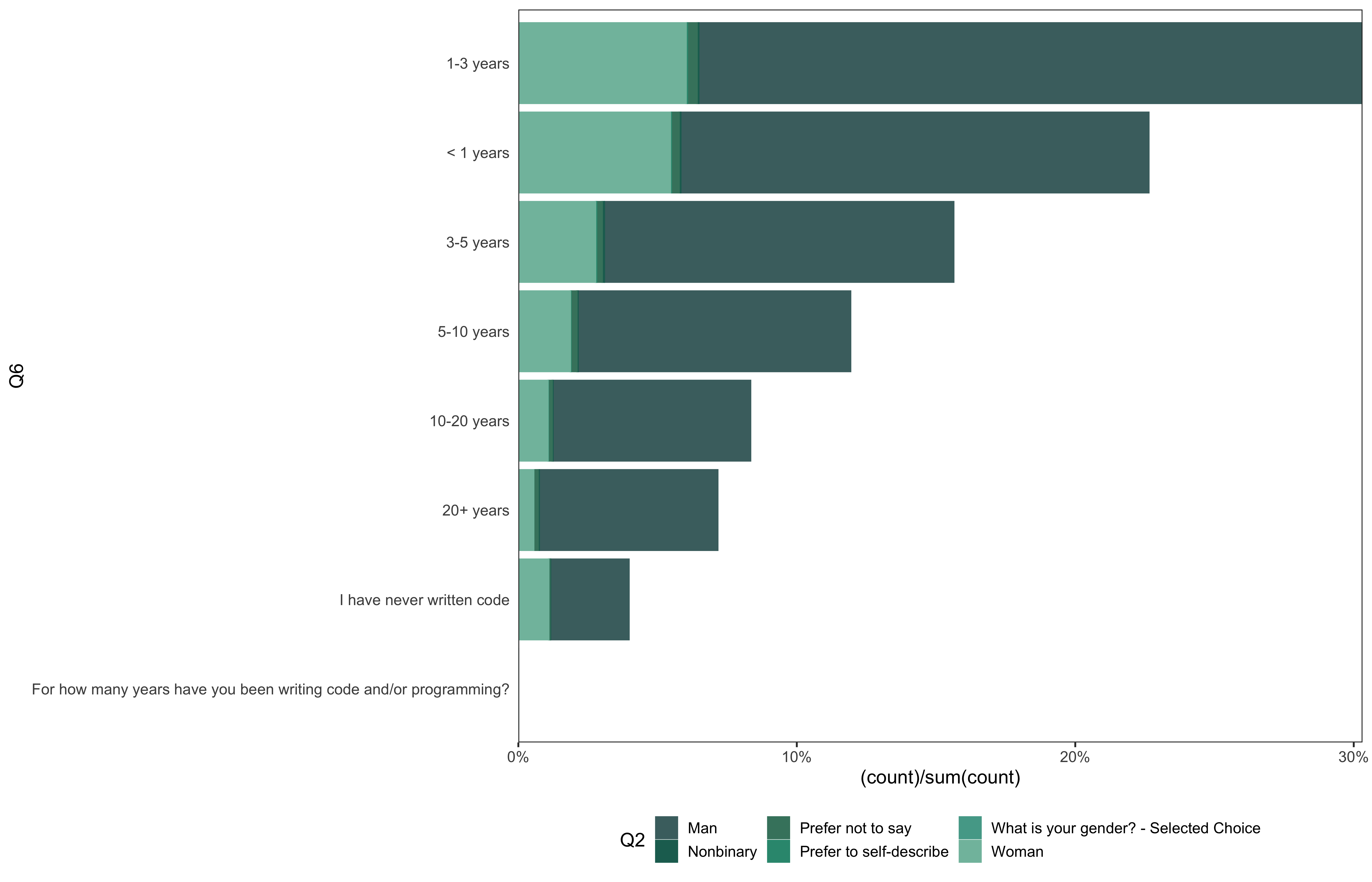
data %>%
  go(Q6)
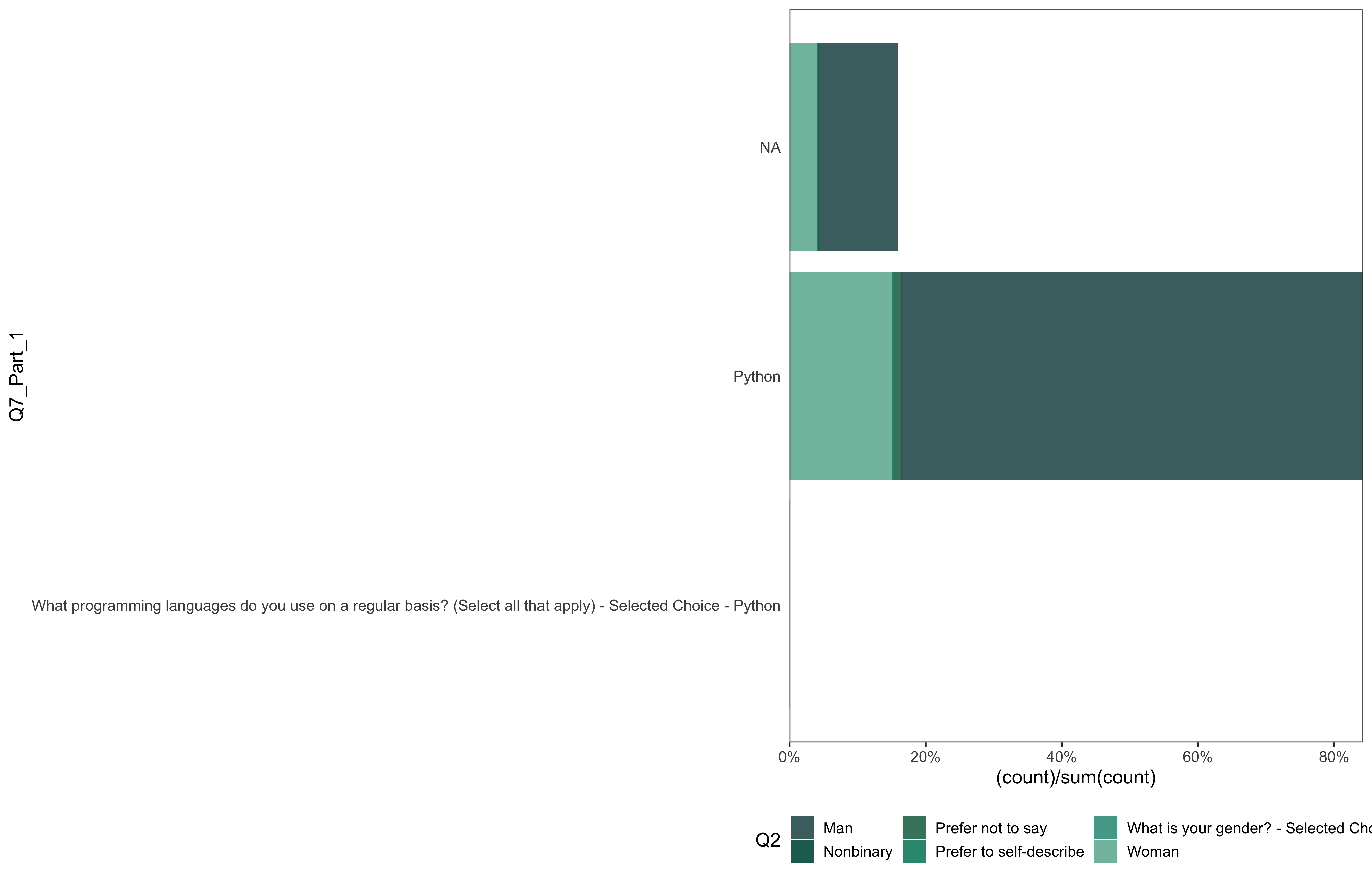
# mutually exclusive answers
data %>%
  go(Q7_Part_1)
data %>%
  go(Q7_Part_2)

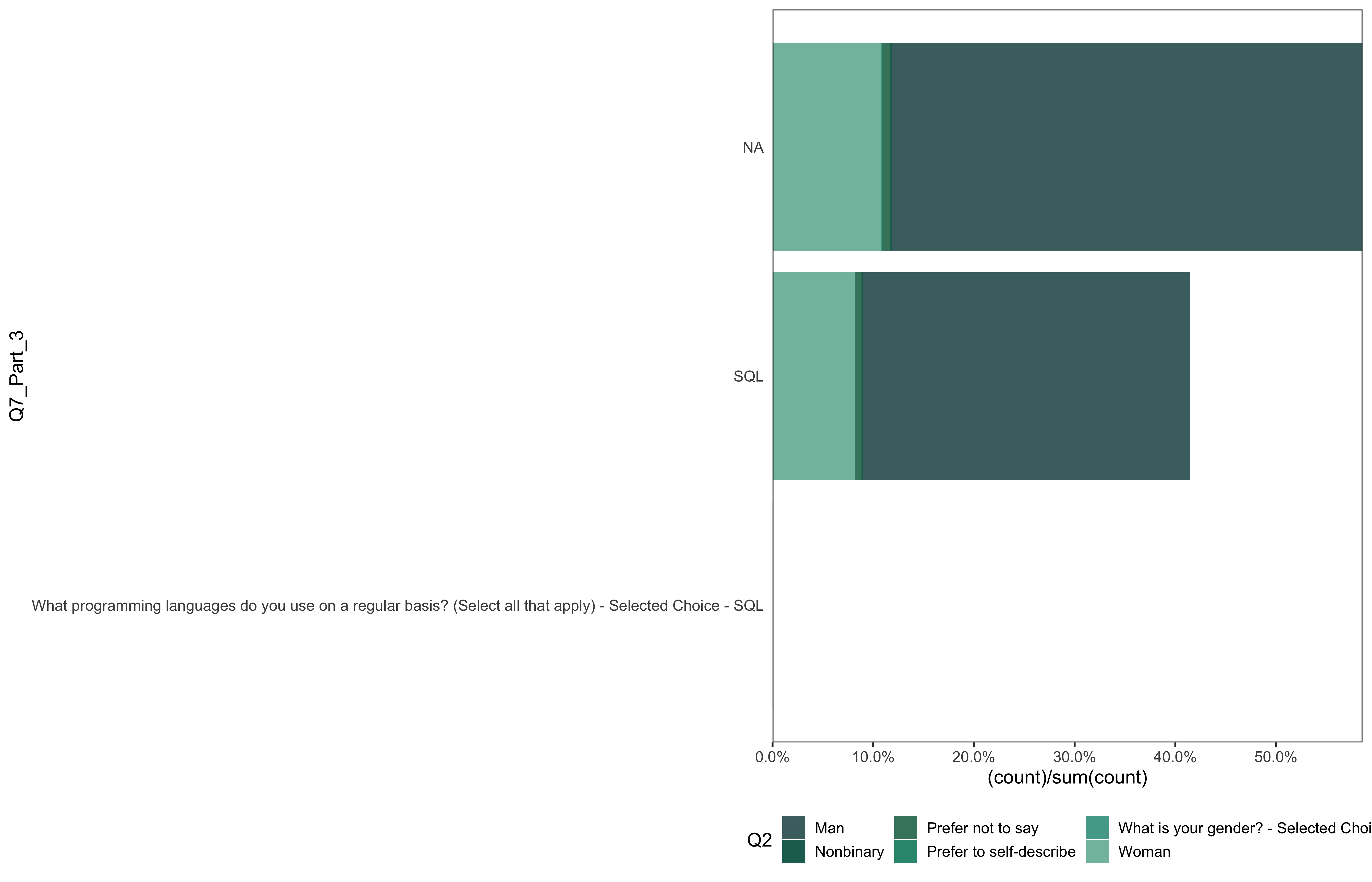
data %>%
  go(Q7_Part_3)
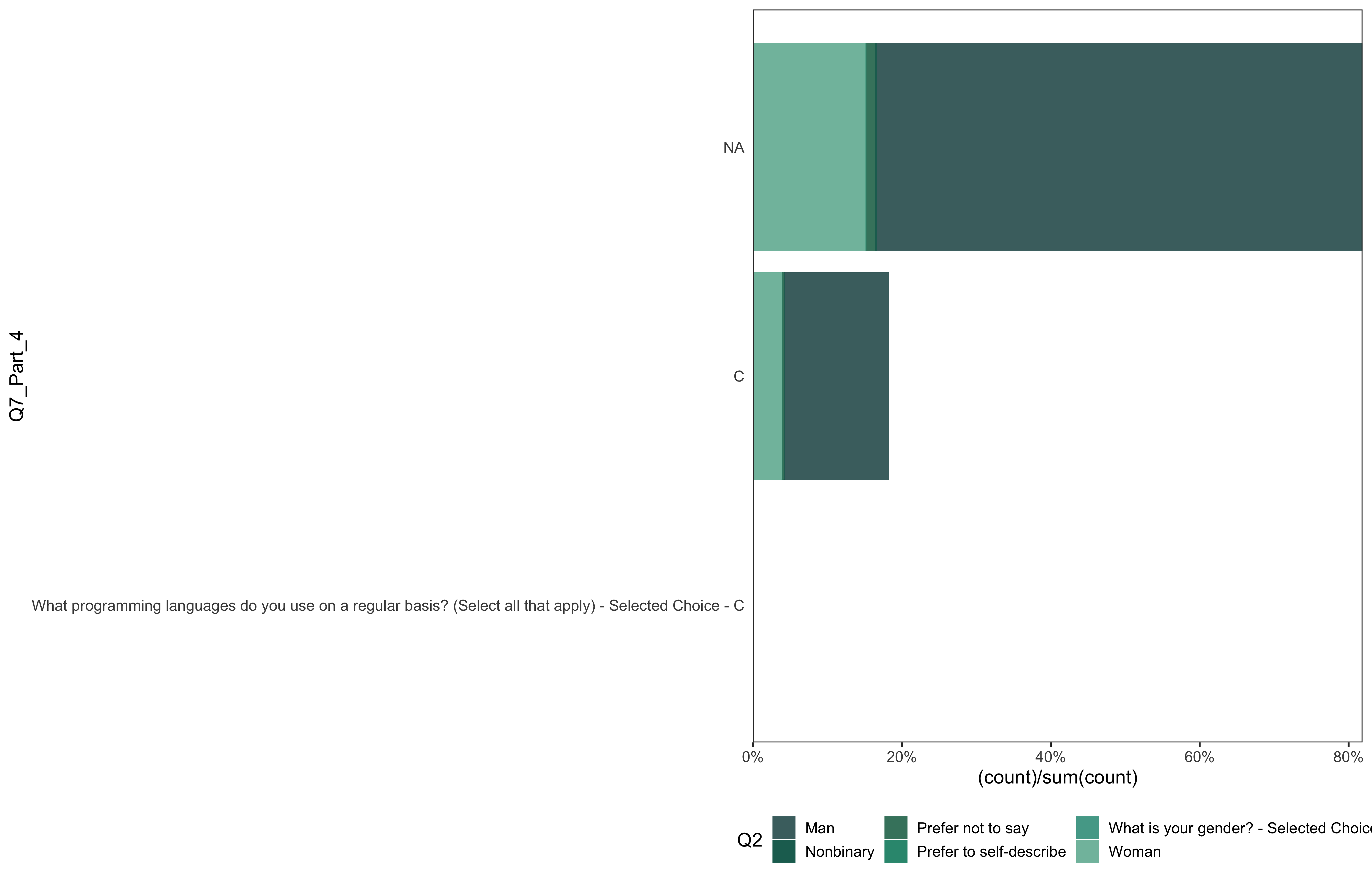
data %>%
  go(Q7_Part_4)
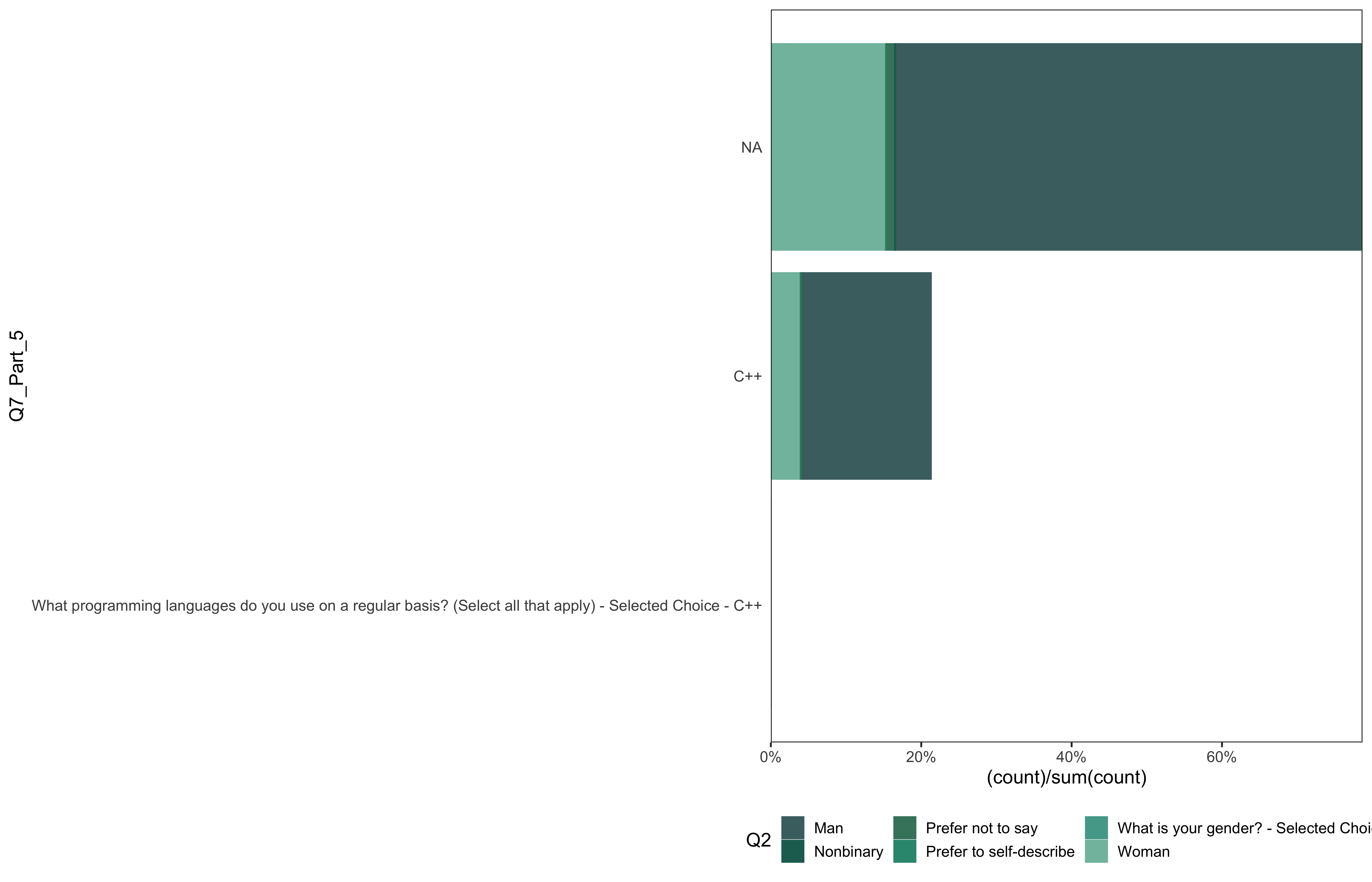
data %>%
  go(Q7_Part_5)
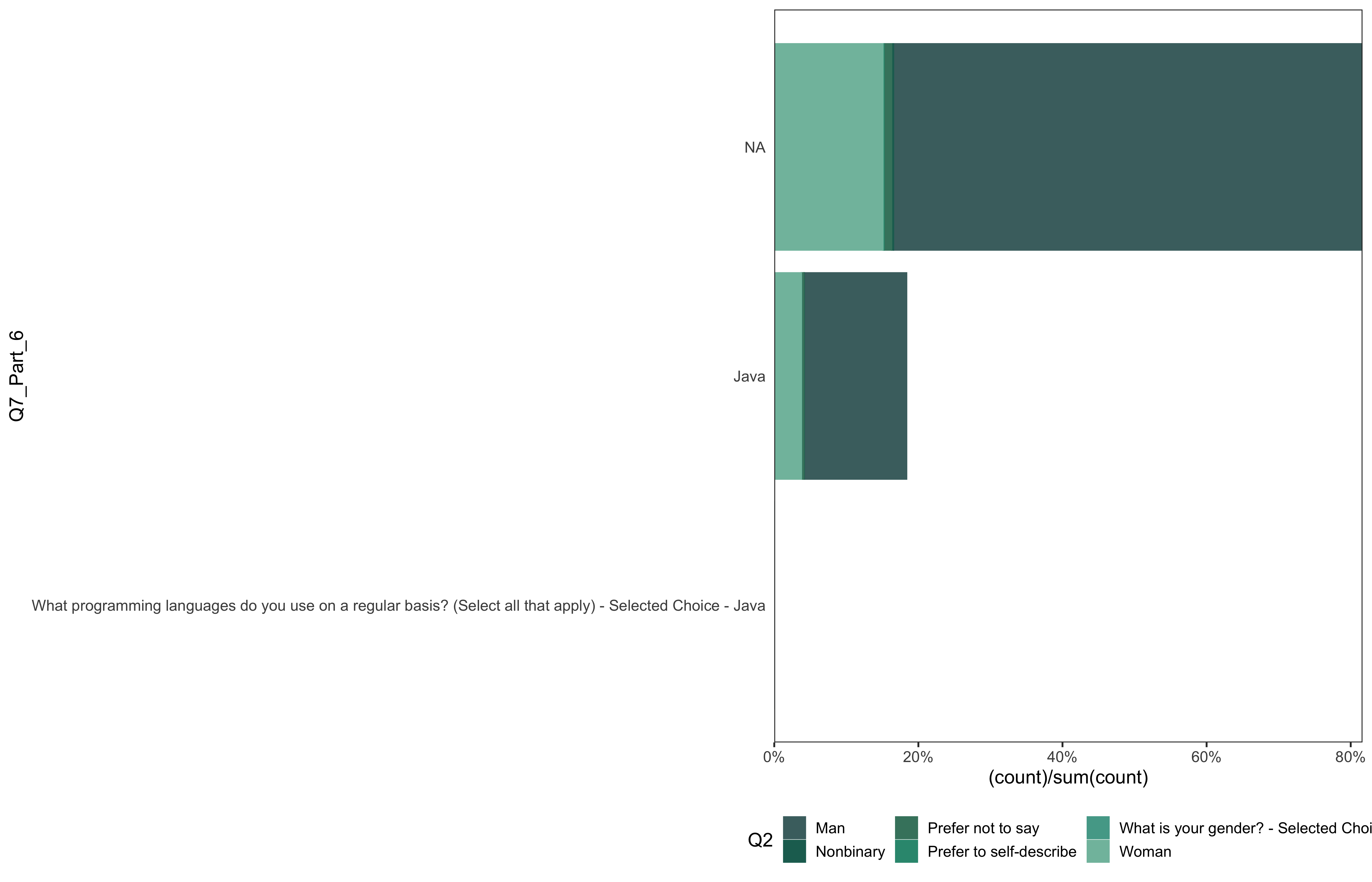
data %>%
  go(Q7_Part_6)
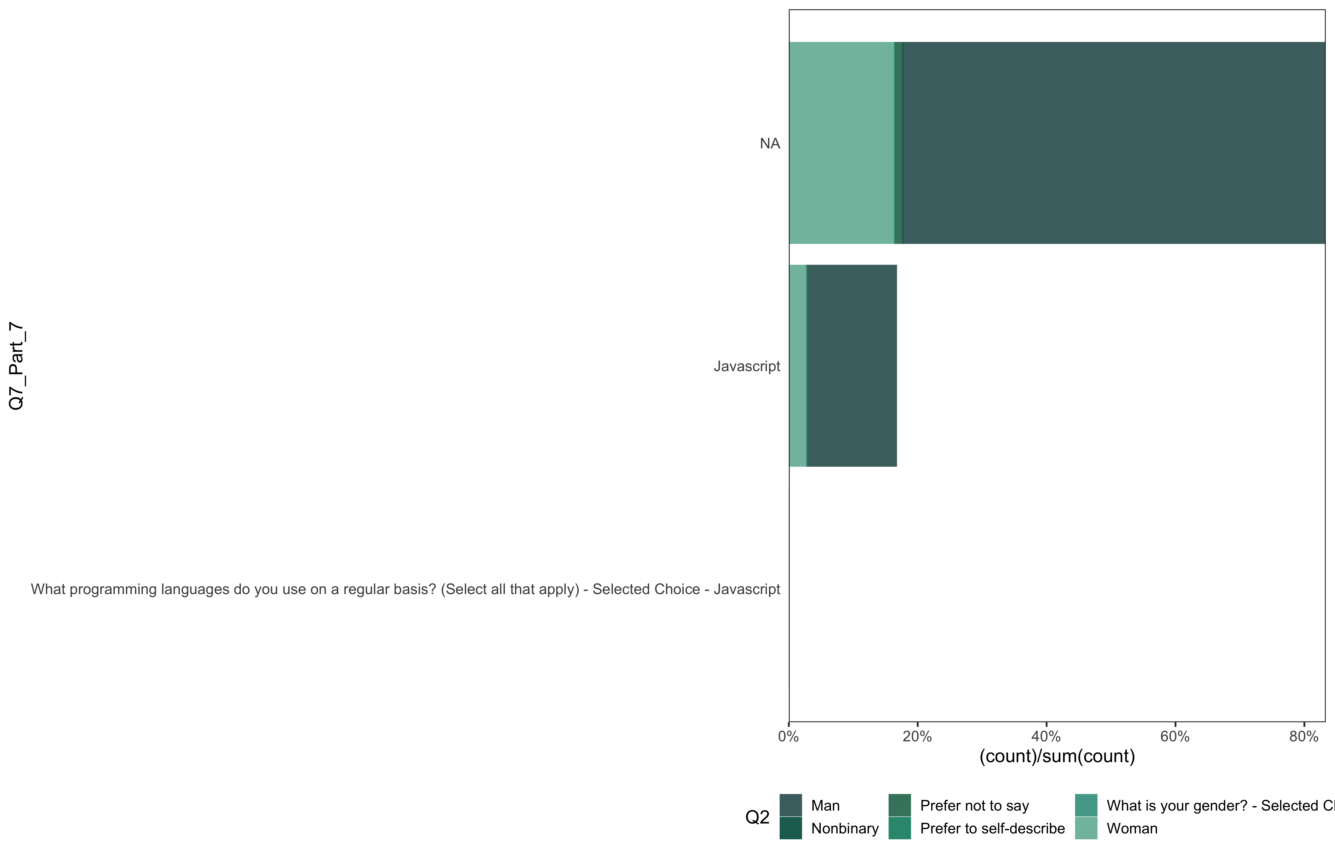
data %>%
  go(Q7_Part_7)
data_2 <-
  data %>%
  select(Q2, Q7_Part_1:Q7_OTHER) %>%
  filter(row_number() != 1) %>%
  unite(col = "Q7", Q7_Part_1:Q7_Part_7, sep = ", ", na.rm = T) %>%
  filter(Q7 != "")

data_2 %>%
  count(Q7)
## # A tibble: 124 × 2
##    Q7                           n
##    <chr>                    <int>
##  1 C                          129
##  2 C, C++                     111
##  3 C, C++, Java                49
##  4 C, C++, Java, Javascript     5
##  5 C, C++, Javascript          13
##  6 C, Java                     30
##  7 C, Java, Javascript          7
##  8 C, Javascript                6
##  9 C++                        130
## 10 C++, Java                   25
## # … with 114 more rows
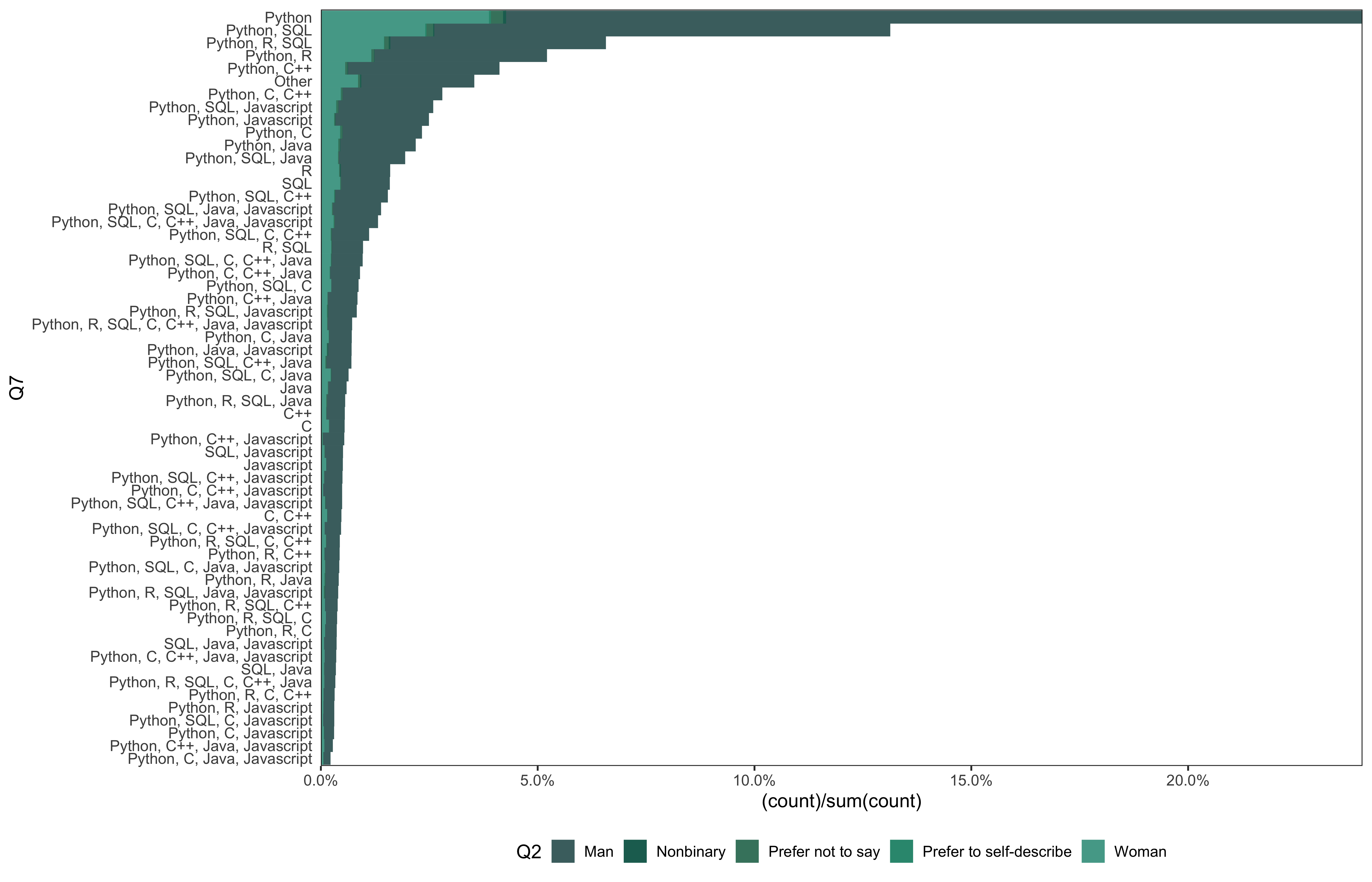
data_2 %>%
  mutate(
    Q7 = fct_lump_min(Q7, min = 50)
  ) %>%
  go(Q7)
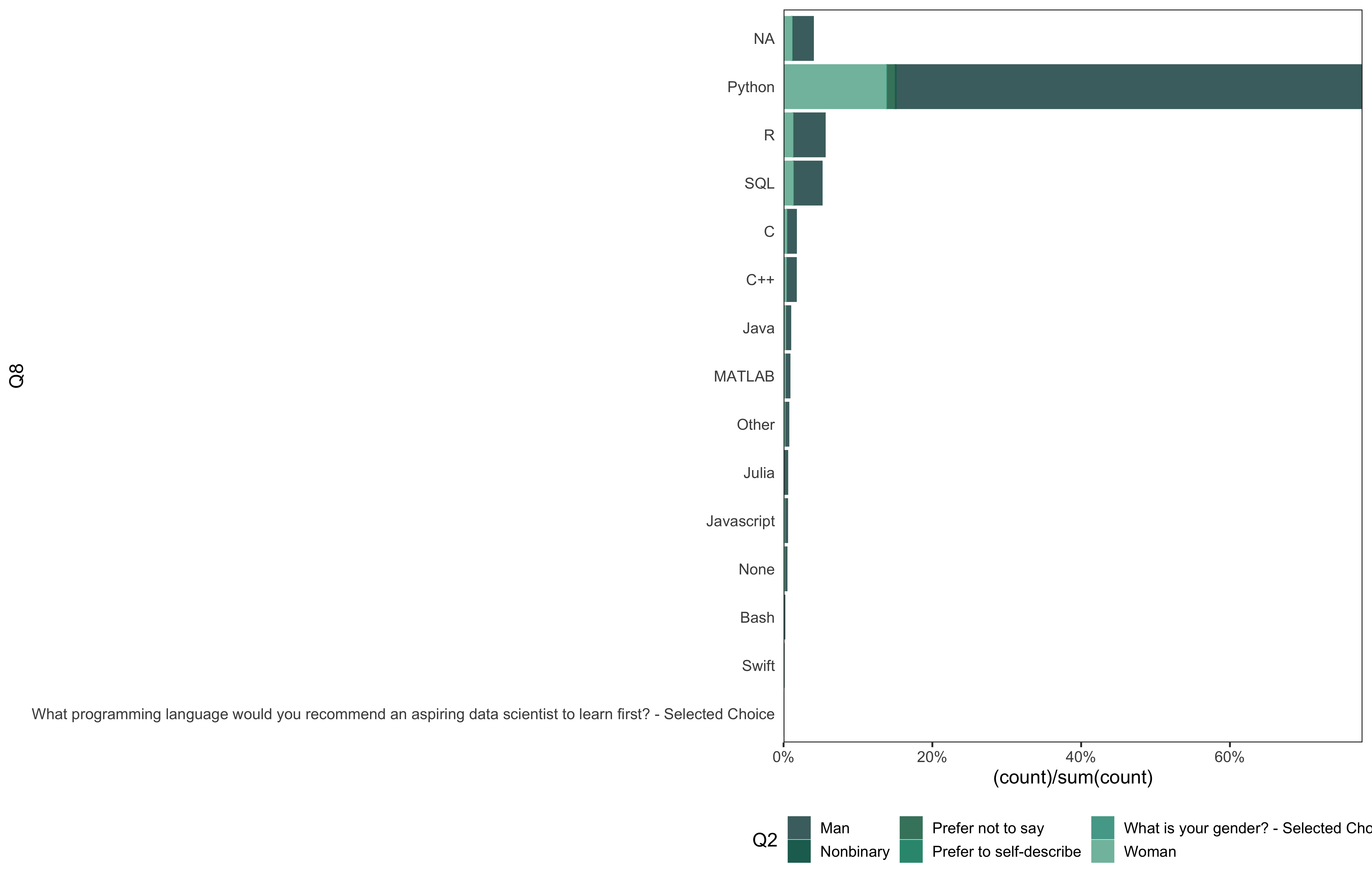
data %>%
  go(Q8)
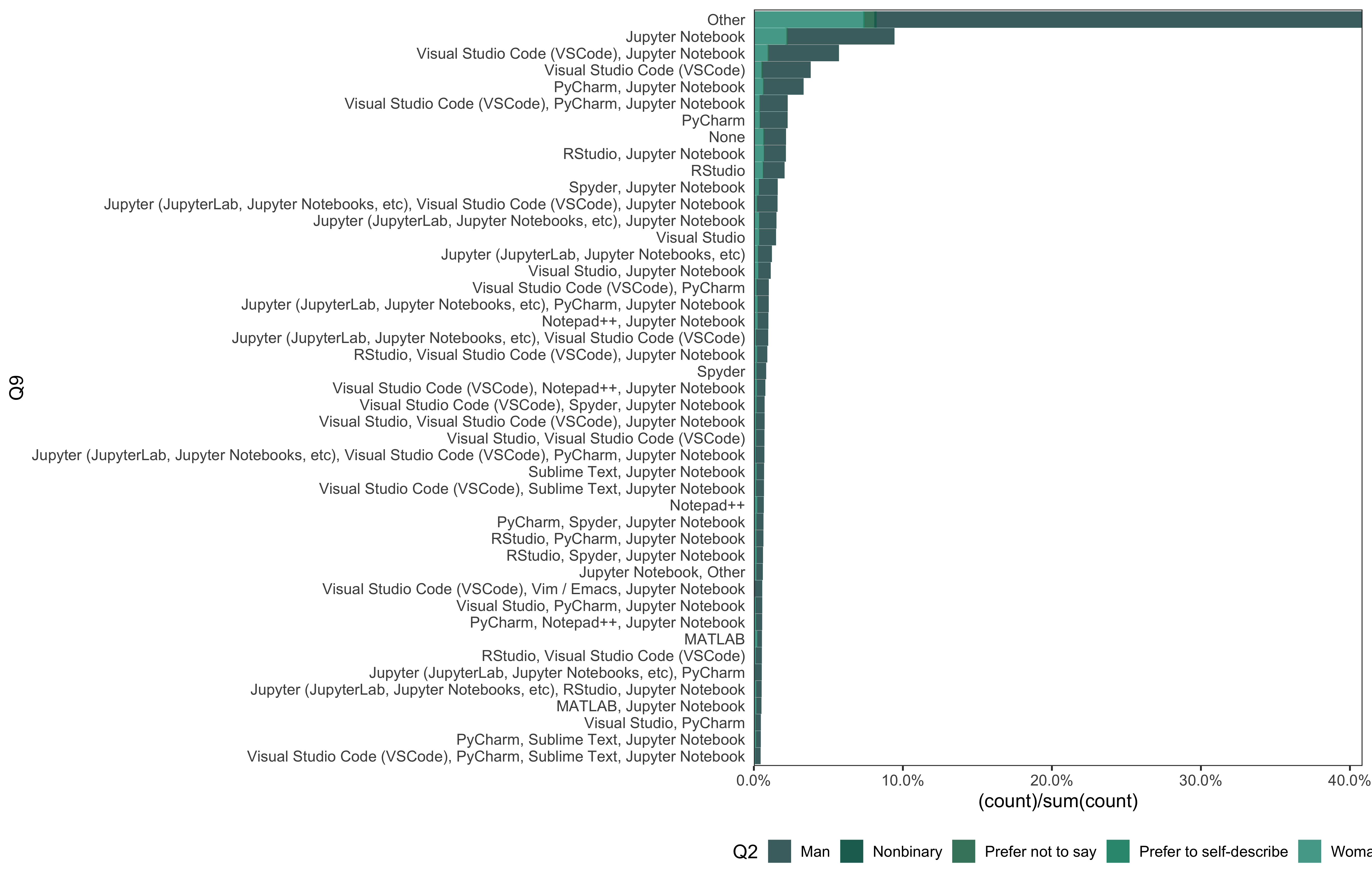
data_3 <-
  data %>%
  select(Q2, Q9_Part_1:Q9_OTHER) %>%
  filter(row_number() != 1) %>%
  unite(col = "Q9", Q9_Part_1:Q9_OTHER, sep = ", ", na.rm = T) %>%
  filter(Q9 != "")

data_3 %>%
  count(Q9)
## # A tibble: 1,330 × 2
##    Q9                                                                          n
##    <chr>                                                                   <int>
##  1 Jupyter (JupyterLab, Jupyter Notebooks, etc)                              290
##  2 Jupyter (JupyterLab, Jupyter Notebooks, etc), Jupyter Notebook            366
##  3 Jupyter (JupyterLab, Jupyter Notebooks, etc), Jupyter Notebook, Other      33
##  4 Jupyter (JupyterLab, Jupyter Notebooks, etc), MATLAB                       11
##  5 Jupyter (JupyterLab, Jupyter Notebooks, etc), MATLAB, Jupyter Notebook     28
##  6 Jupyter (JupyterLab, Jupyter Notebooks, etc), MATLAB, Jupyter Notebook…     3
##  7 Jupyter (JupyterLab, Jupyter Notebooks, etc), Notepad++                    21
##  8 Jupyter (JupyterLab, Jupyter Notebooks, etc), Notepad++, Jupyter Noteb…    61
##  9 Jupyter (JupyterLab, Jupyter Notebooks, etc), Notepad++, Jupyter Noteb…     1
## 10 Jupyter (JupyterLab, Jupyter Notebooks, etc), Notepad++, MATLAB             3
## # … with 1,320 more rows
data_3 %>%
  mutate(
    Q9 = fct_lump_min(Q9, min = 100)
  ) %>%
  go(Q9)
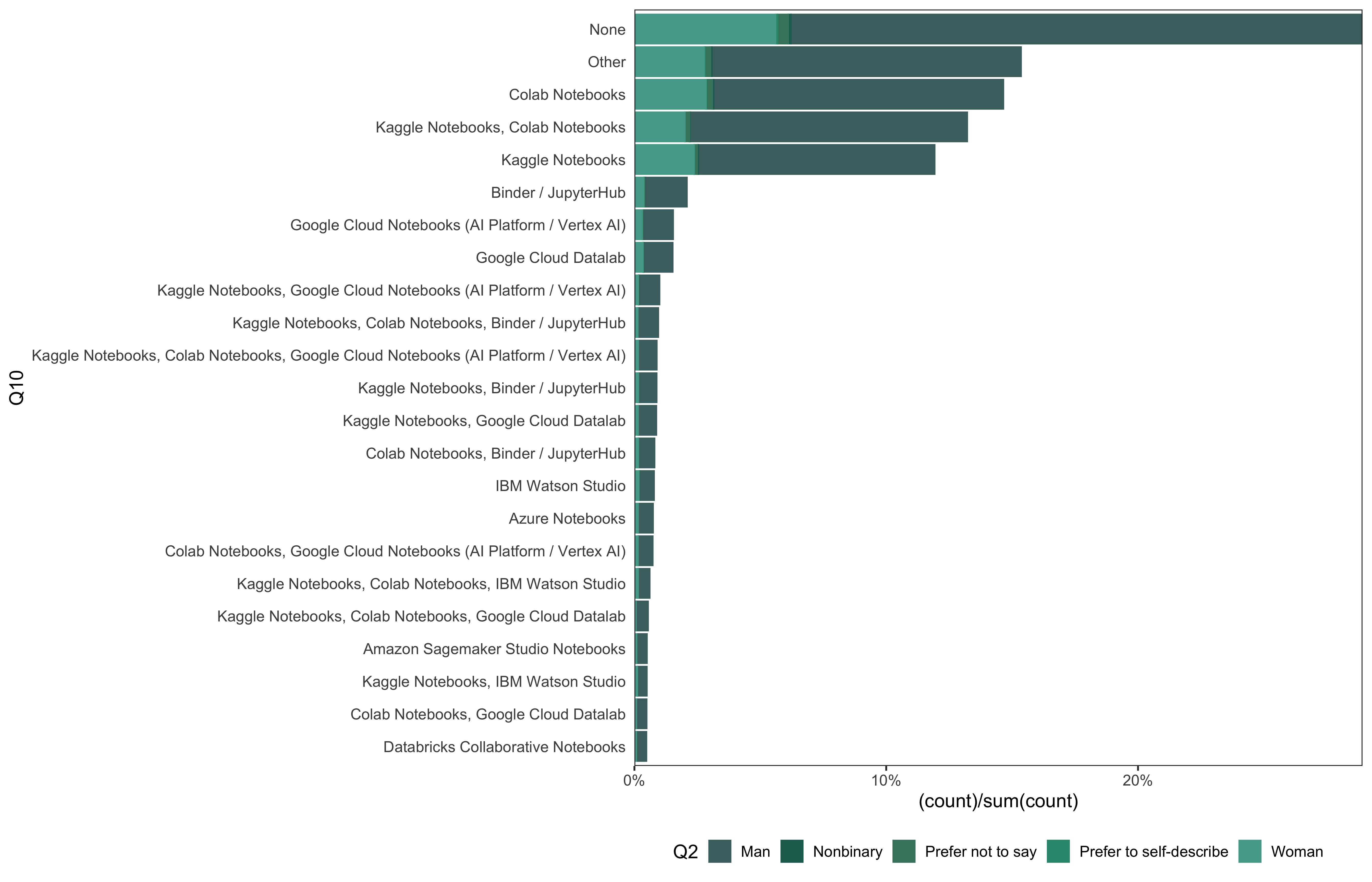
data_4 <-
  data %>%
  select(Q2, Q10_Part_1:Q10_OTHER) %>%
  filter(row_number() != 1) %>%
  unite(col = "Q10", Q10_Part_1:Q10_OTHER, sep = ", ", na.rm = T) %>%
  filter(Q10 != "")

data_4 %>%
  count(Q10)
## # A tibble: 723 × 2
##    Q10                                                                         n
##    <chr>                                                                   <int>
##  1 Amazon EMR Notebooks                                                       40
##  2 Amazon EMR Notebooks, Databricks Collaborative Notebooks                    1
##  3 Amazon EMR Notebooks, Databricks Collaborative Notebooks, Zeppelin / Z…     2
##  4 Amazon EMR Notebooks, Google Cloud Datalab                                  8
##  5 Amazon EMR Notebooks, Google Cloud Notebooks (AI Platform / Vertex AI)      8
##  6 Amazon EMR Notebooks, Google Cloud Notebooks (AI Platform / Vertex AI)…     5
##  7 Amazon EMR Notebooks, Google Cloud Notebooks (AI Platform / Vertex AI)…     1
##  8 Amazon EMR Notebooks, Google Cloud Notebooks (AI Platform / Vertex AI)…     2
##  9 Amazon EMR Notebooks, Other                                                 2
## 10 Amazon EMR Notebooks, Zeppelin / Zepl Notebooks                             3
## # … with 713 more rows
data_4 %>%
  mutate(
    Q10 = fct_lump_min(Q10, min = 100)
  ) %>%
  go(Q10)
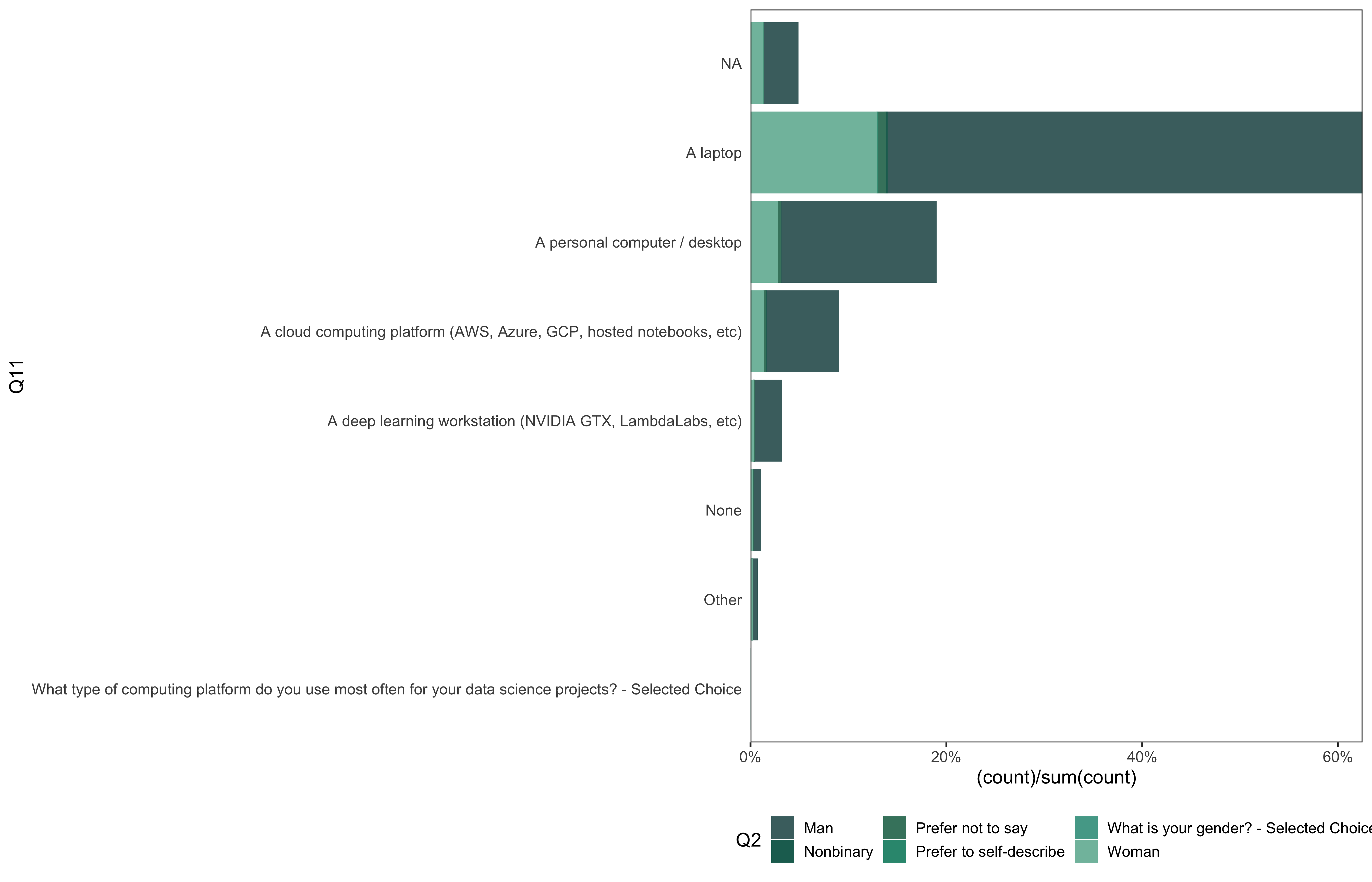
data %>%
  go(Q11)
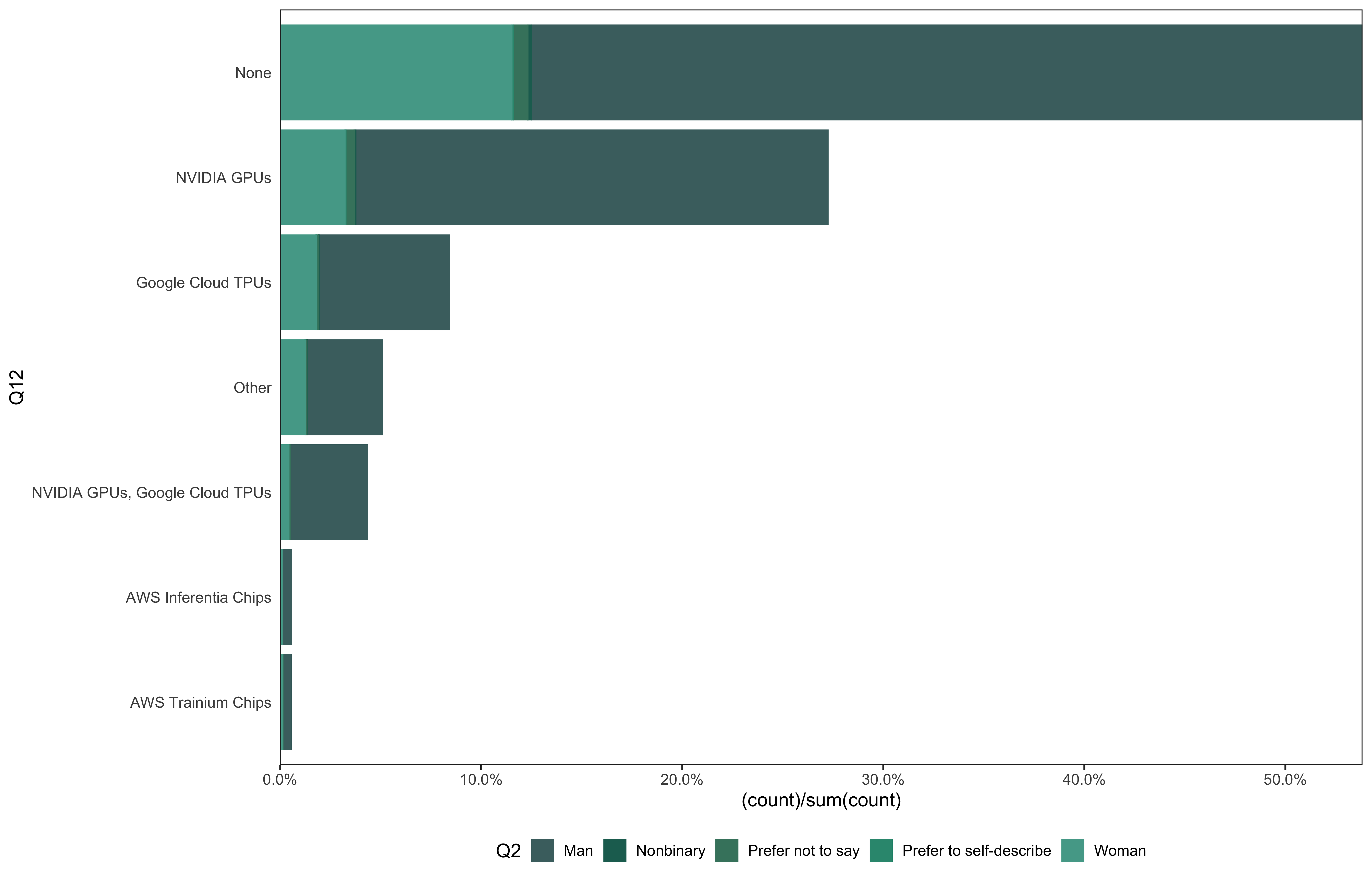
data_5 <-
  data %>%
  select(Q2, Q12_Part_1:Q12_OTHER) %>%
  filter(row_number() != 1) %>%
  unite(col = "Q12", Q12_Part_1:Q12_OTHER, sep = ", ", na.rm = T) %>%
  filter(Q12 != "")

data_5 %>%
  count(Q12)
## # A tibble: 26 × 2
##    Q12                                                             n
##    <chr>                                                       <int>
##  1 AWS Inferentia Chips                                          137
##  2 AWS Inferentia Chips, Other                                     2
##  3 AWS Trainium Chips                                            133
##  4 AWS Trainium Chips, AWS Inferentia Chips                       41
##  5 AWS Trainium Chips, Other                                       1
##  6 Google Cloud TPUs                                            2067
##  7 Google Cloud TPUs, AWS Inferentia Chips                        52
##  8 Google Cloud TPUs, AWS Trainium Chips                          51
##  9 Google Cloud TPUs, AWS Trainium Chips, AWS Inferentia Chips    35
## 10 Google Cloud TPUs, AWS Trainium Chips, Other                    2
## # … with 16 more rows
data_5 %>%
  mutate(
    Q12 = fct_lump_min(Q12, min = 100)
  ) %>%
  go(Q12)
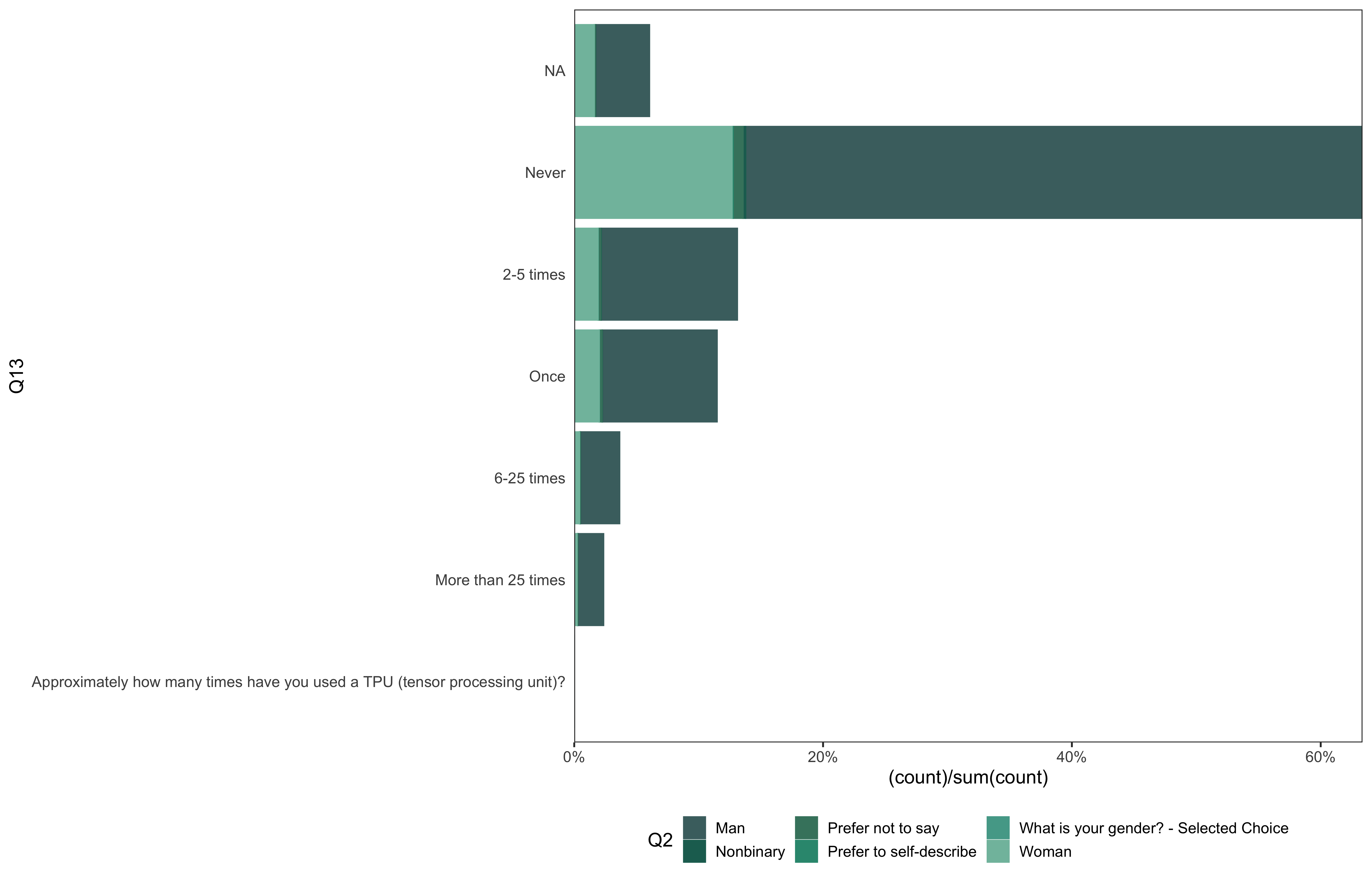
data %>%
  go(Q13)
data_6 <-
  data %>%
  select(Q2, Q14_Part_1:Q14_OTHER) %>%
  filter(row_number() != 1) %>%
  unite(col = "Q14", Q14_Part_1:Q14_OTHER, sep = ", ", na.rm = T) %>%
  filter(Q14 != "")

data_6 %>%
  count(Q14)
## # A tibble: 467 × 2
##    Q14                                     n
##    <chr>                               <int>
##  1 Altair                                 21
##  2 Altair, Bokeh, Leaflet / Folium         1
##  3 Altair, Geoplotlib                      1
##  4 Altair, Leaflet / Folium                2
##  5 Altair, Other                           1
##  6 Bokeh                                  30
##  7 Bokeh, Geoplotlib                       3
##  8 Bokeh, Geoplotlib, Leaflet / Folium     1
##  9 Bokeh, Leaflet / Folium                 2
## 10 Bokeh, Other                            1
## # … with 457 more rows
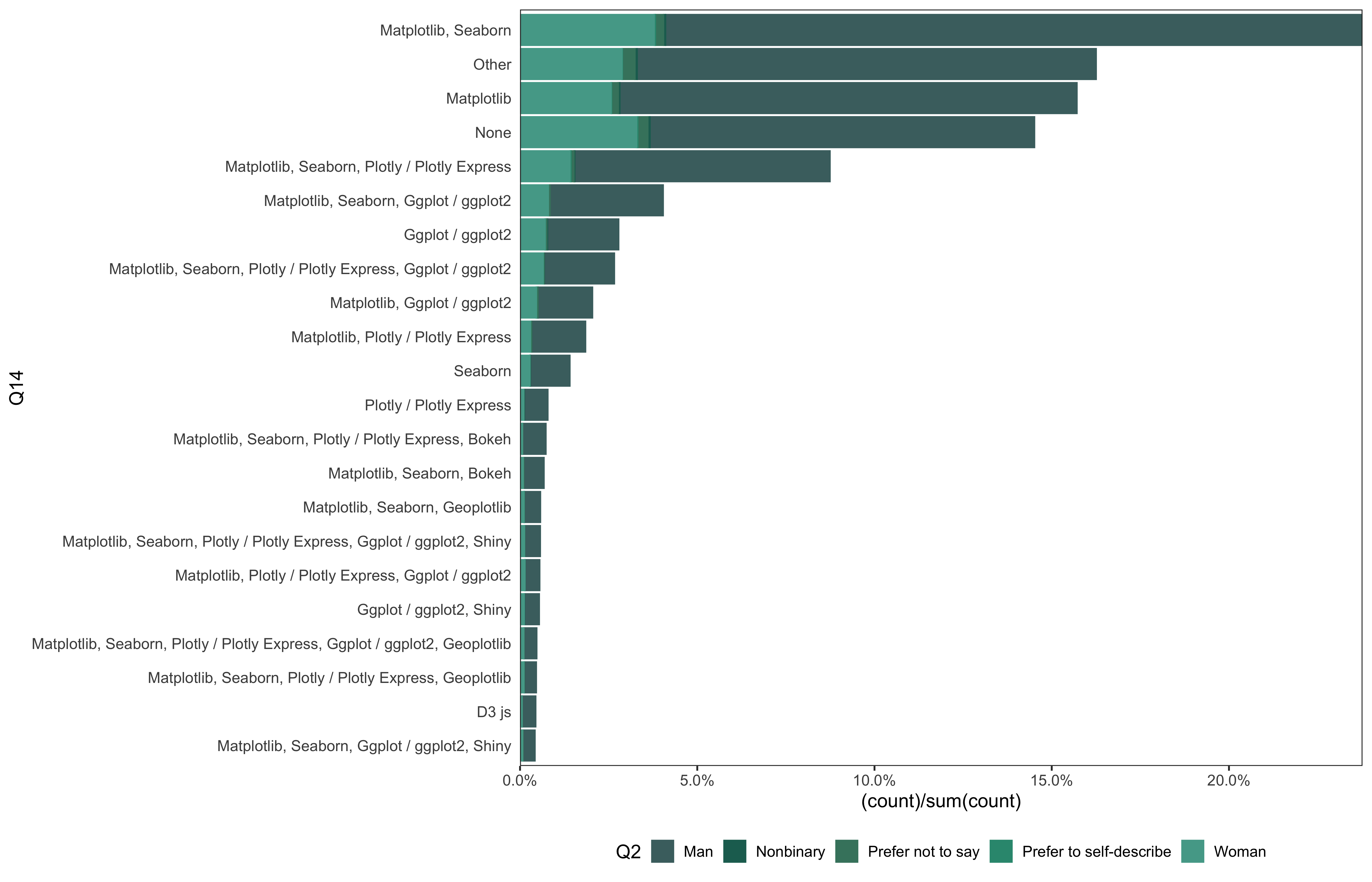
data_6 %>%
  mutate(
    Q14 = fct_lump_min(Q14, min = 100)
  ) %>%
  go(Q14)
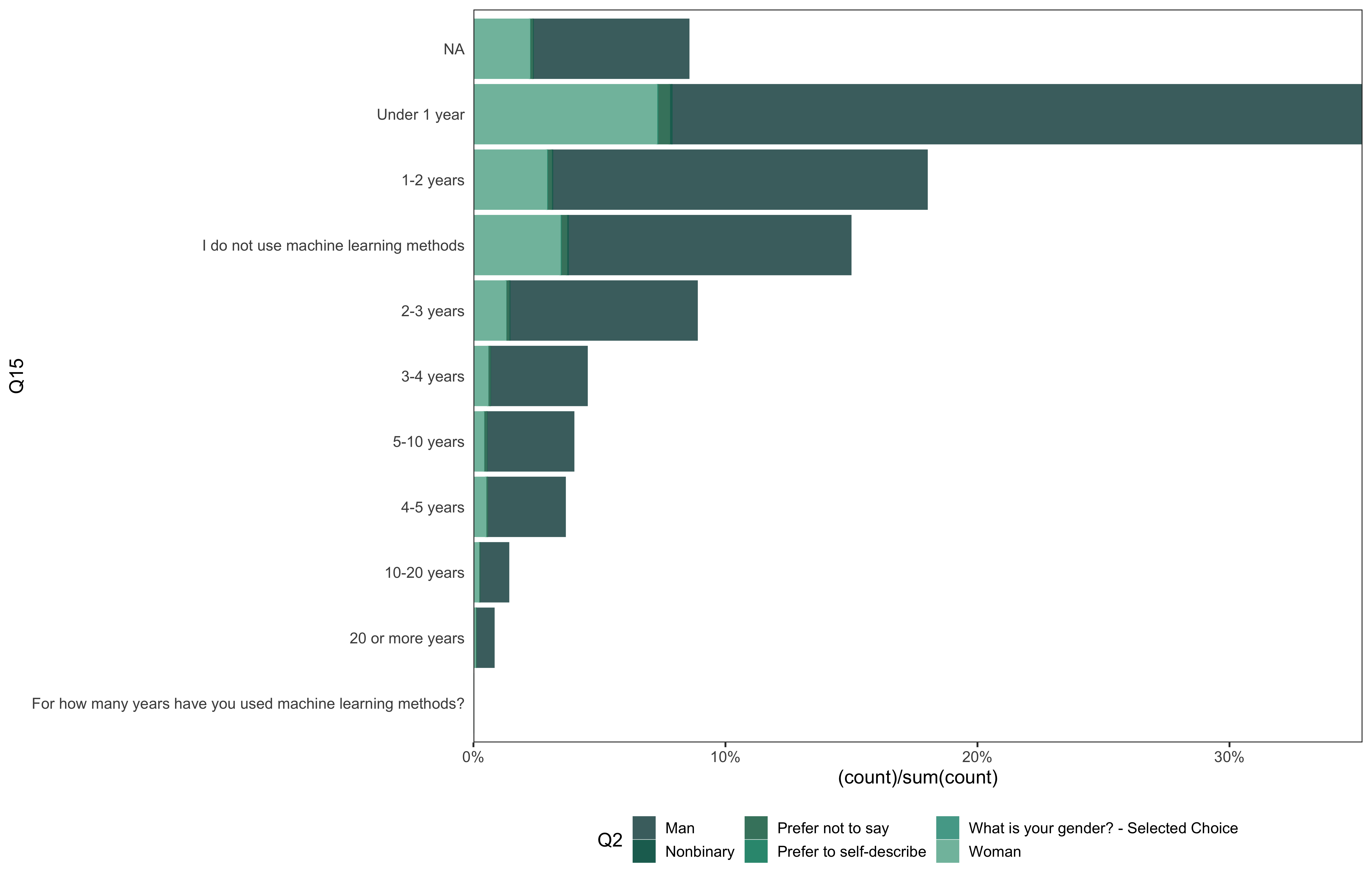
data %>%
  go(Q15)
data_7 <-
  data %>%
  select(Q2, Q16_Part_1:Q16_OTHER) %>%
  filter(row_number() != 1) %>%
  unite(col = "Q16", Q16_Part_1:Q16_OTHER, sep = ", ", na.rm = T) %>%
  filter(Q16 != "")

data_7 %>%
  count(Q16)
## # A tibble: 1,401 × 2
##    Q16                                  n
##    <chr>                            <int>
##  1 Caret                               72
##  2 Caret, Other                         2
##  3 Caret, PyTorch Lightning             1
##  4 Caret, Tidymodels                   35
##  5 CatBoost                            20
##  6 CatBoost, Caret                      1
##  7 CatBoost, Huggingface                1
##  8 CatBoost, JAX                        2
##  9 CatBoost, JAX, PyTorch Lightning     1
## 10 CatBoost, Prophet                    1
## # … with 1,391 more rows
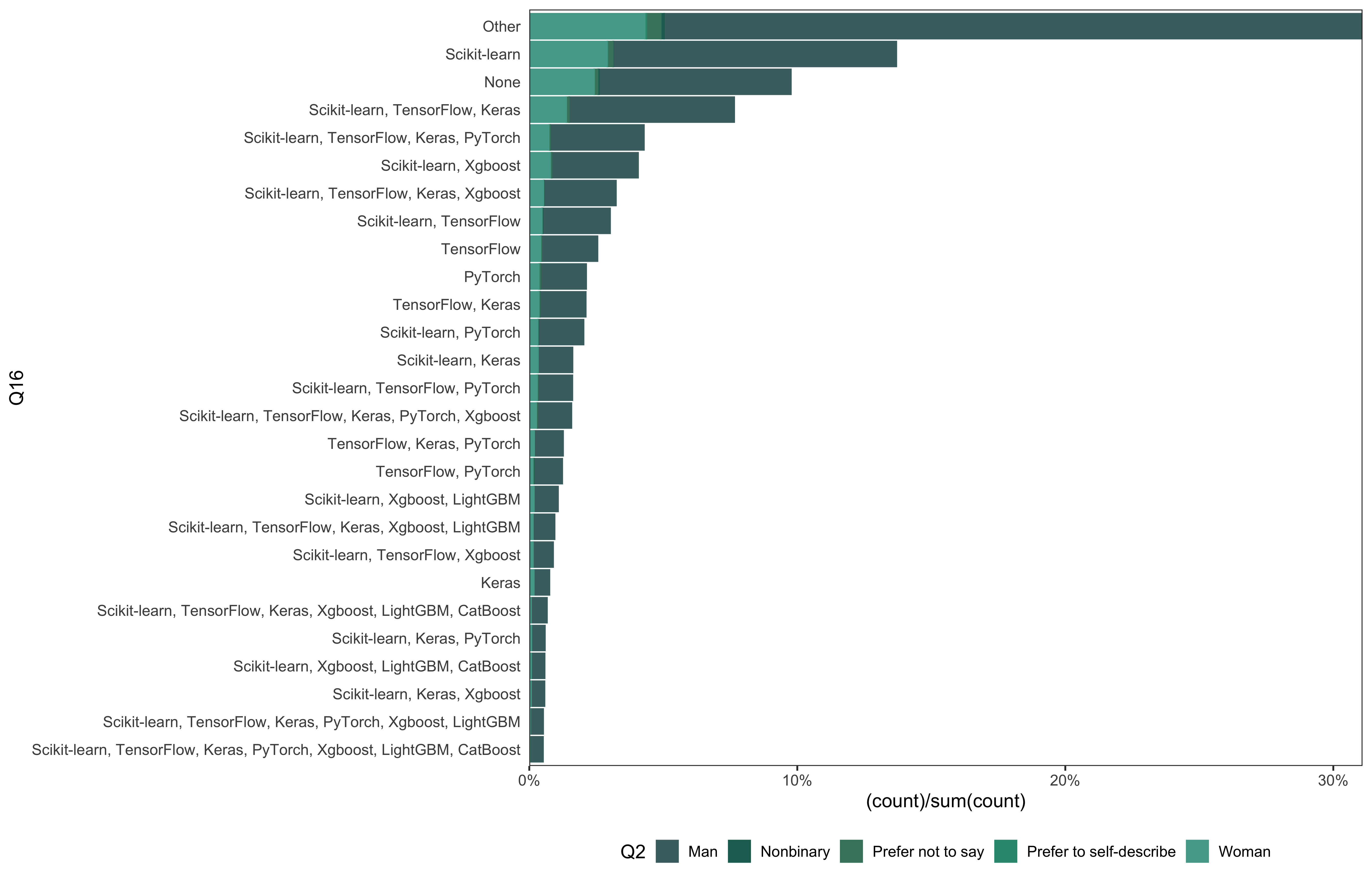
data_7 %>%
  mutate(
    Q16 = fct_lump_min(Q16, min = 100)
  ) %>%
  go(Q16)
data_8 <-
  data %>%
  select(Q2, Q17_Part_1:Q17_OTHER) %>%
  filter(row_number() != 1) %>%
  unite(col = "Q17", Q17_Part_1:Q17_OTHER, sep = ", ", na.rm = T) %>%
  filter(Q17 != "")

data_8 %>%
  count(Q17)
## # A tibble: 756 × 2
##    Q17                                                                         n
##    <chr>                                                                   <int>
##  1 Bayesian Approaches                                                        87
##  2 Bayesian Approaches, Convolutional Neural Networks                         14
##  3 Bayesian Approaches, Convolutional Neural Networks, Generative Adversa…     4
##  4 Bayesian Approaches, Convolutional Neural Networks, Generative Adversa…     1
##  5 Bayesian Approaches, Convolutional Neural Networks, Generative Adversa…     2
##  6 Bayesian Approaches, Convolutional Neural Networks, Recurrent Neural N…    11
##  7 Bayesian Approaches, Convolutional Neural Networks, Recurrent Neural N…     4
##  8 Bayesian Approaches, Convolutional Neural Networks, Transformer Networ…     3
##  9 Bayesian Approaches, Dense Neural Networks (MLPs, etc)                     10
## 10 Bayesian Approaches, Dense Neural Networks (MLPs, etc), Convolutional …     7
## # … with 746 more rows
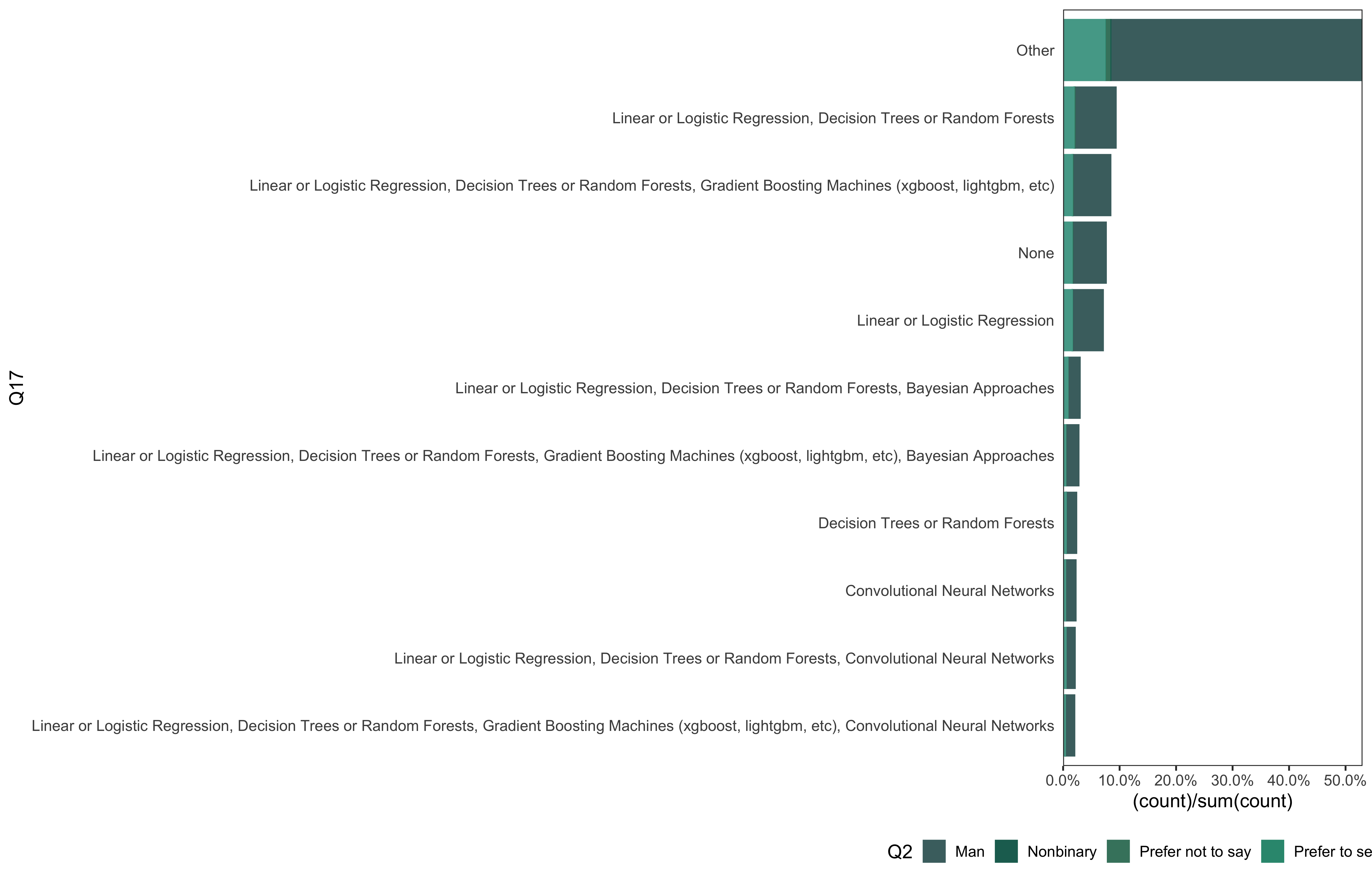
data_8 %>%
  mutate(
    Q17 = fct_lump_min(Q17, min = 300)
  ) %>%
  go(Q17)
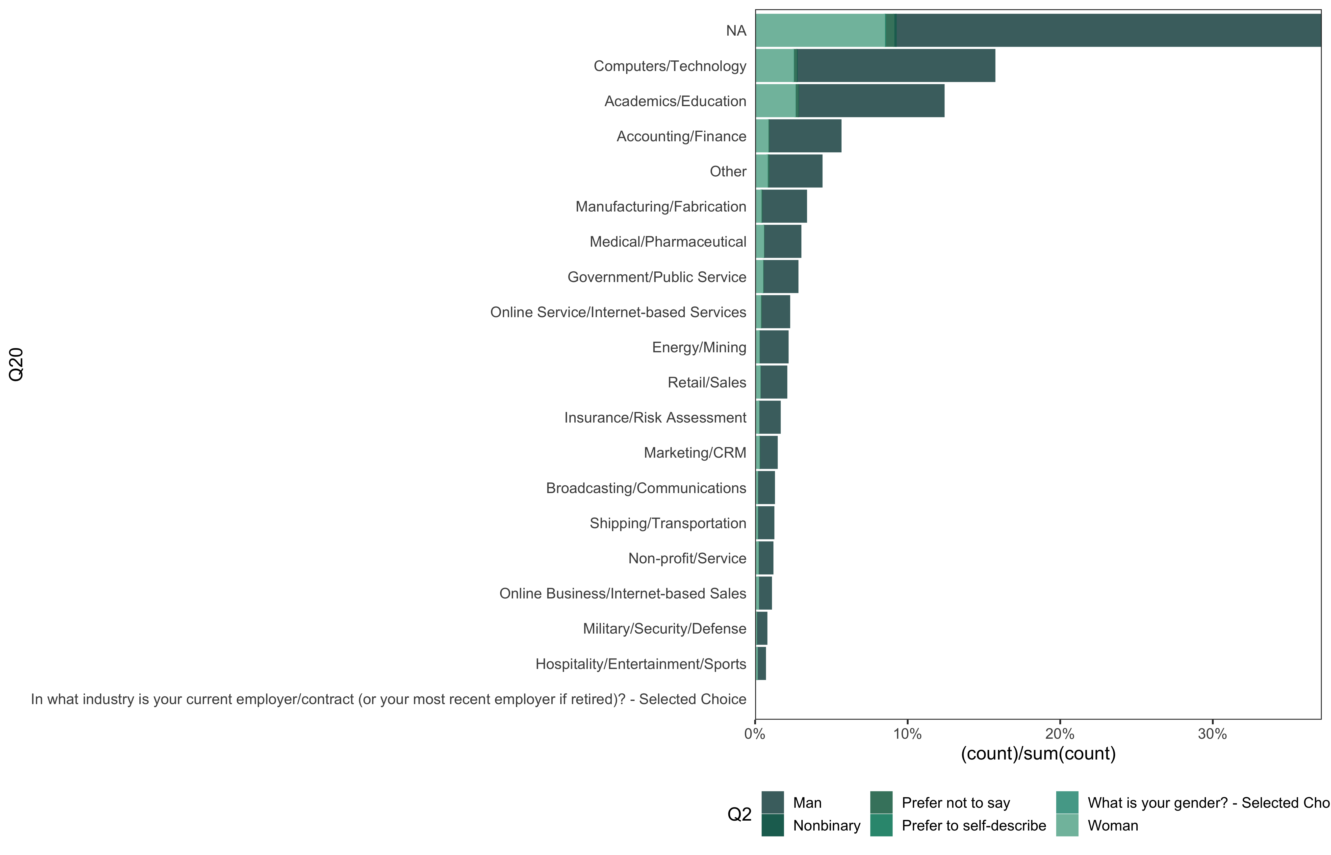
data %>%
  go(Q20)
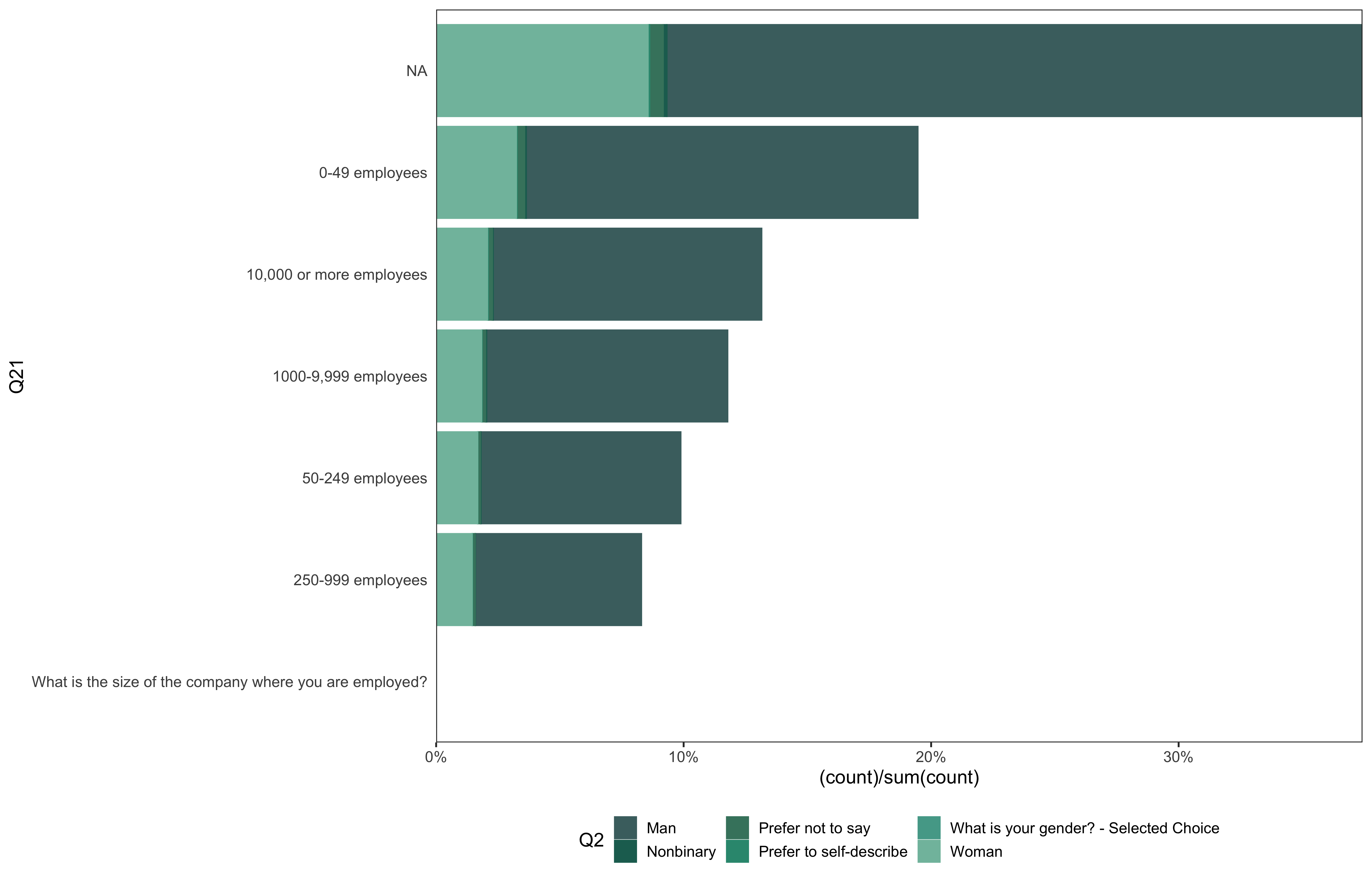
data %>% go(Q21)
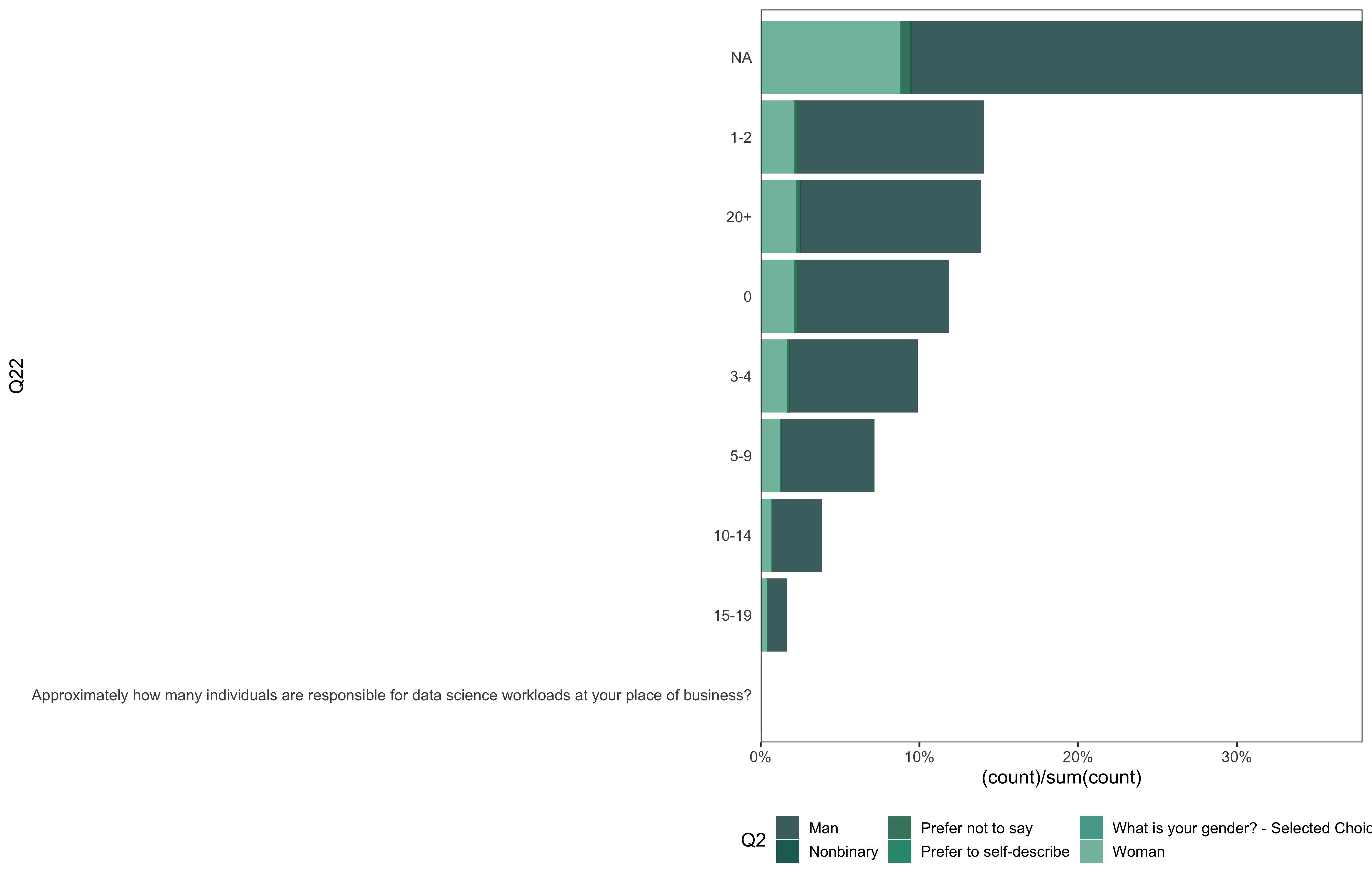
data %>%
  go(Q22)
data %>%
  go(Q25)
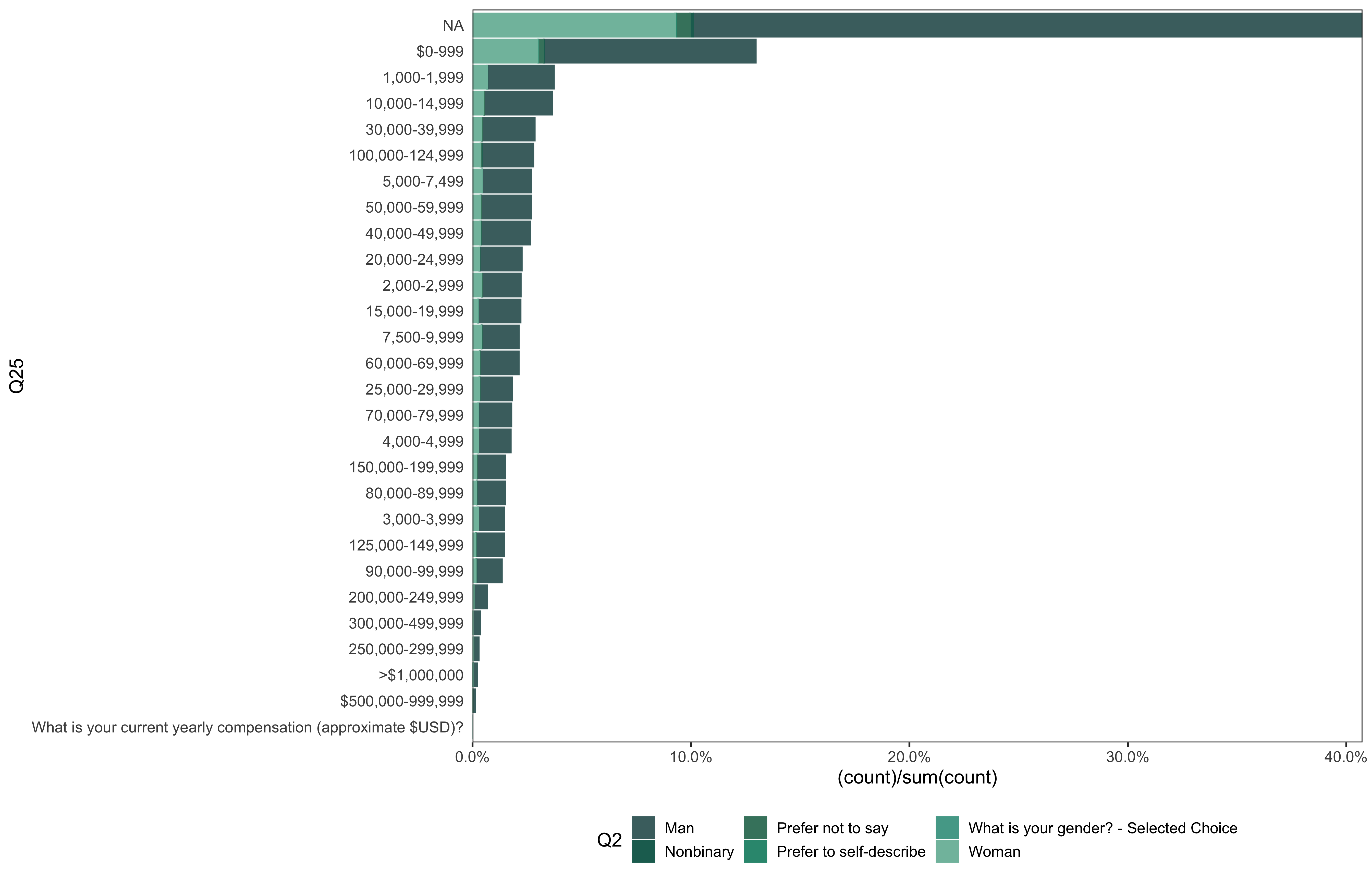
Take home message
- Women and especially non-binary people are still underrepresented in STEM in 2021 and Kaggle survey did not show gender distribution any close to equal.