Antidepressants use in Sweden
Data
Several months have passed since I uploaded Swedish drug utilization data and the structure has changed since then. This time I will focus on antidepressants use in Sweden in more detail 🤓
library(tidyverse)
library(magrittr)
library(wesanderson)
library(RColorBrewer)
regex_antidepress<- "^N06A"
# name the list elements according the name of downloaded .csv files
# path_se is your path with the downloaded and unzipped .csv files
file_names_se<- list.files(path = path_se, pattern = ".csv")
file_names_se
##  [1] "l„kemedel - data - antal expedieringar - 2006-2019.csv"
##  [2] "l„kemedel - data - antal patienter - 2006-2019.csv"
##  [3] "l„kemedel - data - befolkning - 2006-2019.csv"
##  [4] "l„kemedel - data - expedieringar_1000 inv†nare - 2006-2019.csv"
##  [5] "l„kemedel - data - patienter_1000 inv†nare - 2006-2019.csv"
##  [6] "l„kemedel - meta - †ldrar.csv"
##  [7] "l„kemedel - meta - ATC.csv"
##  [8] "l„kemedel - meta - k”n.csv"
##  [9] "l„kemedel - meta - m†tt.csv"
## [10] "l„kemedel - meta - regioner.csv"
# load the data files
all_files_se<- map(file_names_se, ~read_delim(file = paste0(path_se, .x), trim_ws = T, delim = ";")) %>%
  # I expect that formatting of numbers in the files may not be standard; I re-format all columns to character type to deal with numbers' formatting later
  map(~mutate_all(.x, as.character))
Files 1 to 5 now describe each of relevant stat (number of patients, population size, etc.) and files 6 to 10 contain meta-data.
all_files_se[[1]] %>% slice(1:5)
## # A tibble: 5 × 7
## Mått År Region `ATCkod` Kön Ålder Värde
## <chr> <chr> <chr> <chr> <chr> <chr> <chr>
## 1 3 2006 0 TOTALT 1 1 560858
## 2 3 2006 0 TOTALT 1 2 413587
## 3 3 2006 0 TOTALT 1 3 415480
## 4 3 2006 0 TOTALT 1 4 474248
## 5 3 2006 0 TOTALT 1 5 444933
# Note the region coded as character 0, 1, 2
# age categories
all_files_se[[6]] %>% slice(1:5)
## # A tibble: 5 × 2
##   Ålder Text
##   <chr> <chr>
## 1 1     0-4
## 2 2     5-9
## 3 3     10-14
## 4 4     15-19
## 5 5     20-24
# ATC codes
all_files_se[[7]] %>% slice(1:5)
## # A tibble: 5 × 2
##   ATC    Text
##   <chr>  <chr>
## 1 TOTALT Samtliga (A - V)
## 2 A      Matsmältningsorgan och ämnesomsättning
## 3 A01    Medel vid mun- och tandsjukdomar
## 4 A01A   Medel vid mun- och tandsjukdomar
## 5 A01AA  Medel mot karies
# sex labels
all_files_se[[8]] %>% slice(1:5)
## # A tibble: 3 × 2
##   Kön   Text
##   <chr> <chr>
## 1 1     Män
## 2 2     Kvinnor
## 3 3     Båda könen
# stats
all_files_se[[9]] %>% slice(1:5)
## # A tibble: 5 × 2
##   Mått  Text
##   <chr> <chr>
## 1 1     Antal patienter
## 2 2     Patienter/1000 invånare
## 3 3     Antal expedieringar
## 4 4     Expedieringar/1000 invånare
## 5 9     Befolkning
# 1 - Number of patients: 2 - Patients per 1000 inhabitants; 3 - Number of dispensings; 4 - Dispensings per 1000 inhabitants; 9 - Population
# region
all_files_se[[10]] %>% slice(1:5)
## # A tibble: 5 × 2
##   Region Text
##   <chr>  <chr>
## 1 00     Riket
## 2 01     Stockholms län
## 3 03     Uppsala län
## 4 04     Södermanlands län
## 5 05     Östergötlands län
# Note the region coded as 00, 01, 02 in the meta-data file and 0, 1, 2 in the files with stats --> recode

all_files_se[[10]]  %<>% mutate(
    Region = parse_integer(Region)
  )
data_se<- bind_rows(all_files_se[c(1:5)]) %>%
  # join with age groups labels
  left_join(all_files_se[[6]]) %>%
  # rename joined column to age_group
  rename(age_group = Text) %>%
  # rename ATCkod to ATC
  rename(ATC = 4) %>%
  # keep only ATC codes of interest
  filter(str_detect(string = ATC, pattern = regex_antidepress)) %>%
  # join with drugs labels
  left_join(all_files_se[[7]]) %>%
  # rename joined column
  rename(drug = Text) %>%
  # join with sex labels
  left_join(all_files_se[[8]]) %>%
  # rename joined column
  rename(gender = Text) %>%
  # keep records on drug utilization in women
  filter(gender == "Kvinnor") %>%
  # join with characteristics' labels
  left_join(all_files_se[[9]]) %>%
  # rename characteristics' labels column
  rename(stat = Text) %>%
  # regions as integer
  mutate(
    Region = parse_integer(Region)
  ) %>%
  # join with regions' labels column
  left_join(all_files_se[[10]]) %>%
  # rename regions' labels column
  rename(region_text = Text) %>%
  # keep stats for the whole country
  filter(region_text == "Riket") %>%
  # rename some of the columns in the data while selecting columns in the desired order
  select(year = År,
         region = region_text,
         ATC,
         values = Värde,
         age_group,
         drug,
         gender,
         stat)

data_se %>% slice(1:5)
## # A tibble: 5 × 8
##   year  region ATC   values age_group drug                 gender  stat
##   <chr> <chr>  <chr> <chr>  <chr>     <chr>                <chr>   <chr>
## 1 2006  Riket  N06A  10     0-4       Antidepressiva medel Kvinnor Antal expedi…
## 2 2006  Riket  N06A  118    5-9       Antidepressiva medel Kvinnor Antal expedi…
## 3 2006  Riket  N06A  2729   10-14     Antidepressiva medel Kvinnor Antal expedi…
## 4 2006  Riket  N06A  29828  15-19     Antidepressiva medel Kvinnor Antal expedi…
## 5 2006  Riket  N06A  64871  20-24     Antidepressiva medel Kvinnor Antal expedi…
Time to put these data into wide format so that each stats has its own column to work with.
# pivot data into wide format so that each stat has its column
data_se %<>% pivot_wider(names_from = stat, values_from = values) %>%
  # format numbers using with dot as a decimal separator
  mutate(
    `Expedieringar/1000 invånare` = str_replace_all(string = `Expedieringar/1000 invånare`, pattern = ",", replacement = "."),
    `Patienter/1000 invånare` = str_replace_all(string = `Patienter/1000 invånare`, pattern = ",", replacement = "."),
    `Expedieringar/1000 invånare` = as.numeric(`Expedieringar/1000 invånare`),
    `Patienter/1000 invånare` = as.numeric(`Patienter/1000 invånare`)
  ) %>%
  # all to numeric
  mutate_at(vars(`Antal expedieringar`, `Antal patienter`, Befolkning, year), as.numeric)

data_se %>% slice(1:5)
## # A tibble: 5 × 11
##    year region ATC   age_group drug     gender `Antal expedier… `Antal patiente…
##   <dbl> <chr>  <chr> <chr>     <chr>    <chr>             <dbl>            <dbl>
## 1  2006 Riket  N06A  0-4       Antidep… Kvinn…               10               10
## 2  2006 Riket  N06A  5-9       Antidep… Kvinn…              118               38
## 3  2006 Riket  N06A  10-14     Antidep… Kvinn…             2729              758
## 4  2006 Riket  N06A  15-19     Antidep… Kvinn…            29828             7794
## 5  2006 Riket  N06A  20-24     Antidep… Kvinn…            64871            15396
## # … with 3 more variables: Befolkning <dbl>, Expedieringar/1000 invånare <dbl>,
## #   Patienter/1000 invånare <dbl>
I am interested in adults under 85 only, and I will keep the original age categorization.
data_se %>% distinct(age_group)
## # A tibble: 19 × 1
##    age_group
##    <chr>
##  1 0-4
##  2 5-9
##  3 10-14
##  4 15-19
##  5 20-24
##  6 25-29
##  7 30-34
##  8 35-39
##  9 40-44
## 10 45-49
## 11 50-54
## 12 55-59
## 13 60-64
## 14 65-69
## 15 70-74
## 16 75-79
## 17 80-84
## 18 85+
## 19 Totalt
# I will negate %in% operator to NOT keep age groups that out of the scope of my interest
data_se %<>% filter(! age_group %in% c("0-4", "5-9", "10-14", "85+", "Totalt"))

data_se %>% distinct(age_group)
## # A tibble: 14 × 1
##    age_group
##    <chr>
##  1 15-19
##  2 20-24
##  3 25-29
##  4 30-34
##  5 35-39
##  6 40-44
##  7 45-49
##  8 50-54
##  9 55-59
## 10 60-64
## 11 65-69
## 12 70-74
## 13 75-79
## 14 80-84
Voila!
Working with ATC codes
Quick check of ATC codes:
data_se %>% distinct(ATC) %>% slice(1:5)
## # A tibble: 5 × 1
##   ATC
##   <chr>
## 1 N06A
## 2 N06AA
## 3 N06AA01
## 4 N06AA02
## 5 N06AA04
For the lack of better option, I will assign labels for ATC codes manually:
data_se %<>% mutate(
  ATC_label = case_when(
    ATC == "N06A" ~ "Antidepressants",
    ATC == "N06AA" ~ "Non-selective monoamine reuptake inhibitors",
    ATC == "N06AA01" ~ "desipramine",
    ATC == "N06AA02" ~ "imipramine",
    ATC == "N06AA03" ~ "imipramine oxide",
    ATC == "N06AA04" ~ "clomipramine",
    ATC == "N06AA05" ~ "opipramol",
    ATC == "N06AA06" ~ "trimipramine",
    ATC == "N06AA07" ~ "lofepramine",
    ATC == "N06AA08" ~ "dibenzepin",
    ATC == "N06AA09" ~ "amitriptyline",
    ATC == "N06AA10" ~ "nortriptyline",
    ATC == "N06AA11" ~ "protriptyline",
    ATC == "N06AA12" ~ "doxepin",
    ATC == "N06AA13" ~ "iprindole",
    ATC == "N06AA14" ~ "melitracen",
    ATC == "N06AA15" ~ "butriptyline",
    ATC == "N06AA16" ~ "dosulepin",
    ATC == "N06AA17" ~ "amoxapine",
    ATC == "N06AA18" ~ "dimetacrine",
    ATC == "N06AA19" ~ "amineptine",
    ATC == "N06AA21" ~ "maprotiline",
    ATC == "N06AA23" ~ "quinupramine",
    ATC == "N06AB" ~ "Selective serotonin reuptake inhibitors",
    ATC == "N06AB02" ~ "zimeldine",
    ATC == "N06AB03" ~ "fluoxetine",
    ATC == "N06AB04" ~ "citalopram",
    ATC == "N06AB05" ~ "paroxetine",
    ATC == "N06AB06" ~ "sertraline",
    ATC == "N06AB07" ~ "alaproclate",
    ATC == "N06AB08" ~ "fluvoxamine",
    ATC == "N06AB09" ~ "etoperidone",
    ATC == "N06AB10" ~ "escitalopram",
    ATC == "N06AF" ~ "Monoamine oxidase inhibitors, non-selective",
    ATC == "N06AF01" ~ "isocarboxazid",
    ATC == "N06AF02" ~ "nialamide",
    ATC == "N06AF03" ~ "phenelzine",
    ATC == "N06AF04" ~ "tranylcypromine",
    ATC == "N06AF05" ~ "iproniazide",
    ATC == "N06AF06" ~ "iproclozide",
    ATC == "N06AG" ~ "Monoamine oxidase A inhibitors",
    ATC == "N06AG02" ~ "moclobemide",
    ATC == "N06AG03" ~ "toloxatone",
    ATC == "N06AX" ~ "Other antidepressants",
    ATC == "N06AX01" ~ "oxitriptan",
    ATC == "N06AX02" ~ "tryptophan",
    ATC == "N06AX03" ~ "mianserin",
    ATC == "N06AX04" ~ "nomifensine",
    ATC == "N06AX05" ~ "trazodone",
    ATC == "N06AX06" ~ "nefazodone",
    ATC == "N06AX07" ~ "minaprine",
    ATC == "N06AX08" ~ "bifemelane",
    ATC == "N06AX09" ~ "viloxazine",
    ATC == "N06AX10" ~ "oxaflozane",
    ATC == "N06AX11" ~ "mirtazapine",
    ATC == "N06AX12" ~ "bupropion",
    ATC == "N06AX13" ~ "medifoxamine",
    ATC == "N06AX14" ~ "tianeptine",
    ATC == "N06AX15" ~ "pivagabine",
    ATC == "N06AX16" ~ "venlafaxine",
    ATC == "N06AX17" ~ "milnacipran",
    ATC == "N06AX18" ~ "reboxetine",
    ATC == "N06AX19" ~ "gepirone",
    ATC == "N06AX21" ~ "duloxetine",
    ATC == "N06AX22" ~ "agomelatine",
    ATC == "N06AX23" ~ "desvenlafaxine",
    ATC == "N06AX24" ~ "vilazodone",
    ATC == "N06AX25" ~ "Hyperici herba",
    ATC == "N06AX26" ~ "vortioxetine",
    ATC == "N06AX27" ~ "esketamine")
)
data_se %>% distinct(ATC_label) %>% slice(1:5)
## # A tibble: 5 × 1
##   ATC_label
##   <chr>
## 1 Antidepressants
## 2 Non-selective monoamine reuptake inhibitors
## 3 desipramine
## 4 imipramine
## 5 clomipramine
Results
I will use ggrepel package to make labels for each of the age groups.
# wrapper around ggplot2 piece of code

# overall antidepressants use
 plot_overall_antidepressants_use<- function(color_scheme = "Blues", n = 14, data_se, regex_atc, name){

  # define the number of colors
  mycolors<- colorRampPalette(brewer.pal(8, color_scheme))(n)

  plot<- data_se %>%
  filter(str_detect(ATC, {{ regex_atc }})) %>%
  filter(`Patienter/1000 invånare` != 0) %>%
  mutate(label = if_else(year == max(year), as.character(age_group), NA_character_)) %>%
  ggplot(aes(x = year, y = `Patienter/1000 invånare`, color = age_group)) +
  geom_path() +
  facet_grid(rows = vars(ATC_label), scales = "free", drop = T) +
  theme_light(base_size = 14) +
  scale_x_continuous(limits = c(2006, 2021), breaks = c(seq(2006, 2019, 6))) +
  scale_color_manual(values = mycolors) +
  theme(plot.caption = element_text(hjust = 0, size = 10),
        legend.position = "none",
        panel.spacing = unit(0.8, "cm")) +
  labs(y = "Female patients\nper 1,000 women in the population", color = "Age group", title = paste0("Overall ", name), subtitle = "utilization in Swedish women by age groups", caption = "dataviz by Elena Dudukina Twitter @evpatora\nSource: sdb.socialstyrelsen.se") +
  ggrepel::geom_label_repel(aes(label = label), na.rm = TRUE, nudge_x = 2, hjust = 0.5, direction = "y", segment.size = 0.1, segment.colour = "black", show.legend = F)

  plot
 }

overall_regex_list<- list("N06A$", "N06AA$", "N06AB$", "N06AF$", "N06AG$", "N06AX$")

overall_names_list<- list("antidepressants", "non-selective monoamine reuptake inhibitors", "selective serotonin reuptake inhibitors", "monoamine oxidase inhibitors, non-selective", "Monoamine oxidase A inhibitors", "other antidepressants")

overall_colors_list <- list("Blues", "Greens", "Oranges", "Purples", "Reds", "Greys")

overall_plots_list<- pmap(list(overall_colors_list, overall_regex_list, overall_names_list), ~ plot_overall_antidepressants_use(color_scheme = ..1, data_se = data_se, regex_atc = ..2, name = ..3))

overall_plots_list
## [[1]]
##
## [[2]]
##
## [[3]]
##
## [[4]]
##
## [[5]]
##
## [[6]]
data_se %>%
  filter(str_detect(ATC, "N06A$")& year == 2019) %>%
  group_by(ATC, ATC_label, age_group) %>%
  summarise(across(`Patienter/1000 invånare`, max)) %>%
  mutate(`Patienter/1000 invånare` = round(`Patienter/1000 invånare`, 0)) %>%
  arrange(-`Patienter/1000 invånare`)
## `summarise()` has grouped output by 'ATC', 'ATC_label'. You can override using the `.groups` argument.
## # A tibble: 14 × 4
## # Groups: ATC, ATC_label [1]
## ATC ATC_label age_group `Patienter/1000 invånare`
## <chr> <chr> <chr> <dbl>
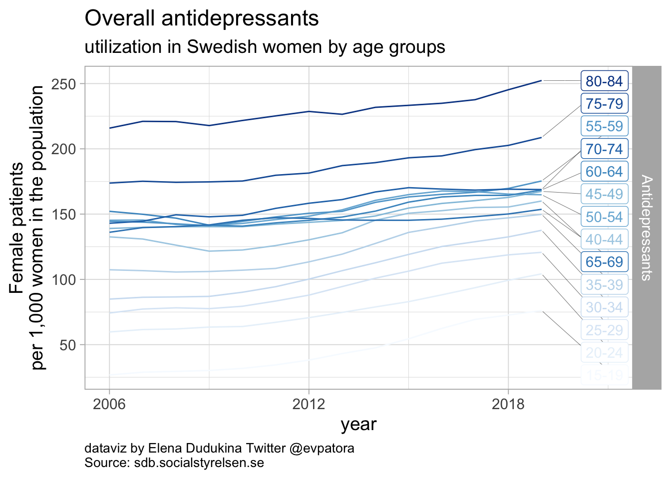
## 1 N06A Antidepressants 80-84 252
## 2 N06A Antidepressants 75-79 209
## 3 N06A Antidepressants 55-59 175
## 4 N06A Antidepressants 70-74 169
## 5 N06A Antidepressants 60-64 168
## 6 N06A Antidepressants 45-49 167
## 7 N06A Antidepressants 50-54 165
## 8 N06A Antidepressants 40-44 160
## 9 N06A Antidepressants 65-69 154
## 10 N06A Antidepressants 35-39 150
## 11 N06A Antidepressants 30-34 138
## 12 N06A Antidepressants 25-29 121
## 13 N06A Antidepressants 20-24 104
## 14 N06A Antidepressants 15-19 76
Overall antidepressants utilization
- Antidepressants utilization was increasing for women of age 70 years and older
- In 2019, the highest rate of overall antidepressant utilization was among women between 80 and 84 years (252 per 1000 women in the population of the same age group)
To have a better understanding of utilization of each of the drugs within each antidepressants class available in Sweden, I will plot utilization for distinct ATC codes between 2006 and 2019 by age groups in 4-year bands.
plot_se_utilization<- function(data, pattern, name, max_year = 2019){
  plot<- data %>%
  filter(str_detect(ATC, {{ pattern }})) %>%
  mutate(label = if_else(year == max_year, as.character(age_group), NA_character_)) %>%
  ggplot(aes(x = year, y = `Patienter/1000 invånare`, color = age_group)) +
  geom_path() +
  theme_light(base_size = 14) +
  scale_x_continuous(limits = c(2006, 2021), breaks = c(seq(2006, 2019, 6))) +
  scale_color_manual(values = wes_palette(name = "Zissou1", n = 14, type = "continuous")) +
  theme(plot.caption = element_text(hjust = 0),
        legend.position = "none",
        panel.spacing = unit(0.8, "cm")) +
  labs(y = "Female patients\nper 1,000 women in the population", color = "Age group", title = paste0(name), subtitle = "Utilization in Swedish women", caption = "dataviz by Elena Dudukina Twitter @evpatora\nSource: sdb.socialstyrelsen.se") +
    ggrepel::geom_label_repel(aes(label = label), na.rm = TRUE, nudge_x = 2, hjust = 0.5, direction = "y", segment.size = 0.1, segment.colour = "black", show.legend = F)

  plot

  }

# construct a list of regular expressions, which capture ATC codes
list_regex<- data_se %>%
  filter(`Patienter/1000 invånare` > 0.1) %>%
   filter(str_detect(ATC, "N06A\\w{1}\\d{2}")) %>%
   distinct(ATC) %>%
   pull()

# construct a list of drug names for each captured ATC code
list_labels<- data_se %>%
  filter(`Patienter/1000 invånare` > 0.1) %>%
   filter(str_detect(ATC, "N06A\\w{1}\\d{2}")) %>%
   distinct(ATC_label) %>%
   pull()

# construct title for the plots
list_names<- map2(list_labels, list_regex, ~ paste0(.x, " (", .y, ")"))

list_plots_se<- map2(list_regex, list_names, ~plot_se_utilization(data = data_se, pattern = .x, name = .y))
list_plots_se[1:5]
## [[1]]
##
## [[2]]
## Warning: ggrepel: 14 unlabeled data points (too many overlaps). Consider
## increasing max.overlaps
##
## [[3]]
##
## [[4]]
##
## [[5]]
## Warning: ggrepel: 12 unlabeled data points (too many overlaps). Consider
## increasing max.overlaps
data_se %>%
  filter(str_detect(ATC, "N06AA\\d{2}")& year == 2019) %>%
  group_by(ATC, ATC_label) %>%
  summarise(across(`Patienter/1000 invånare`, max)) %>%
  mutate(`Patienter/1000 invånare` = round(`Patienter/1000 invånare`, 0))
## # A tibble: 10 × 3
## # Groups:   ATC [10]
##    ATC     ATC_label     `Patienter/1000 invånare`
##    <chr>   <chr>                             <dbl>
##  1 N06AA01 desipramine                           0
##  2 N06AA02 imipramine                            0
##  3 N06AA04 clomipramine                          4
##  4 N06AA05 opipramol                             0
##  5 N06AA06 trimipramine                          0
##  6 N06AA07 lofepramine                           0
##  7 N06AA09 amitriptyline                        33
##  8 N06AA10 nortriptyline                         1
##  9 N06AA11 protriptyline                         0
## 10 N06AA21 maprotiline                           0
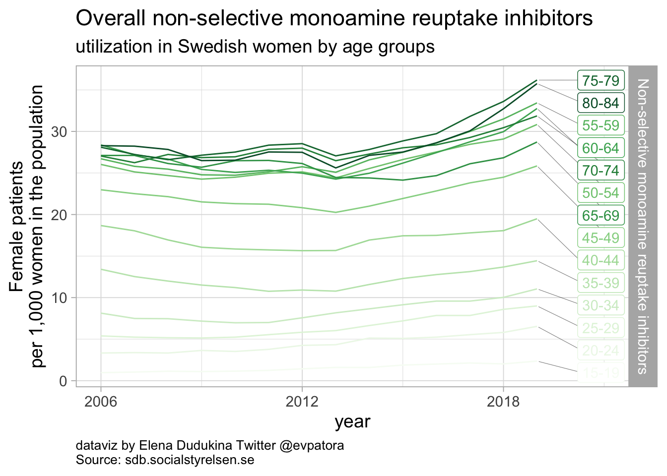
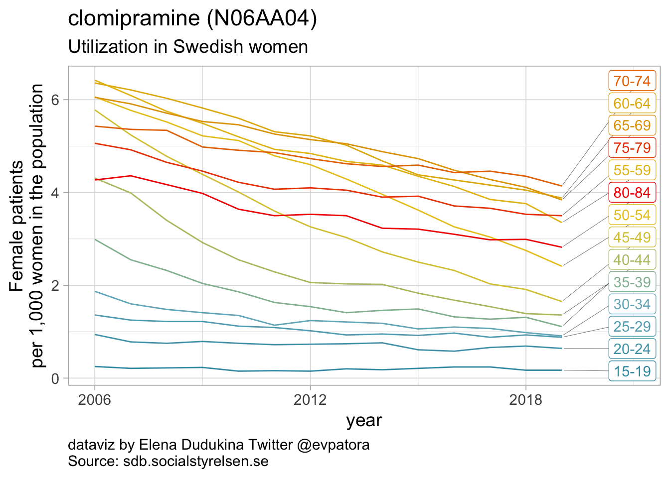
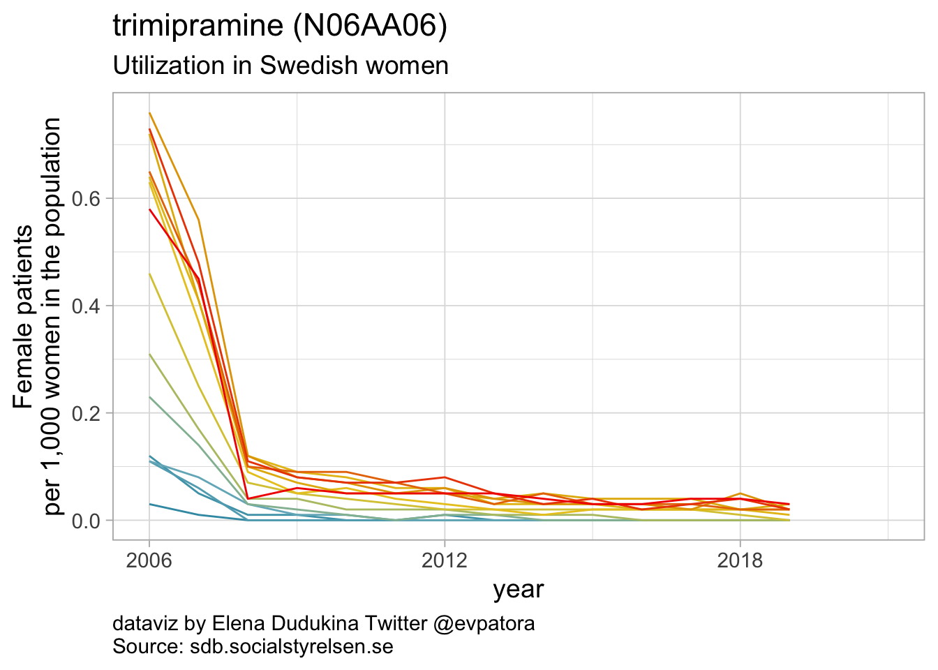
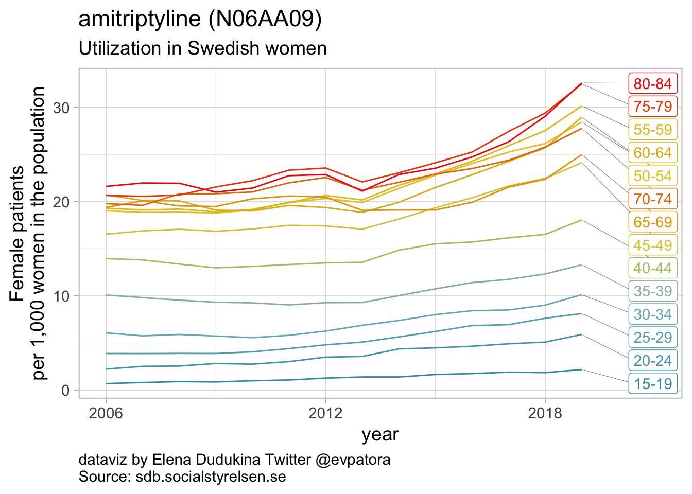
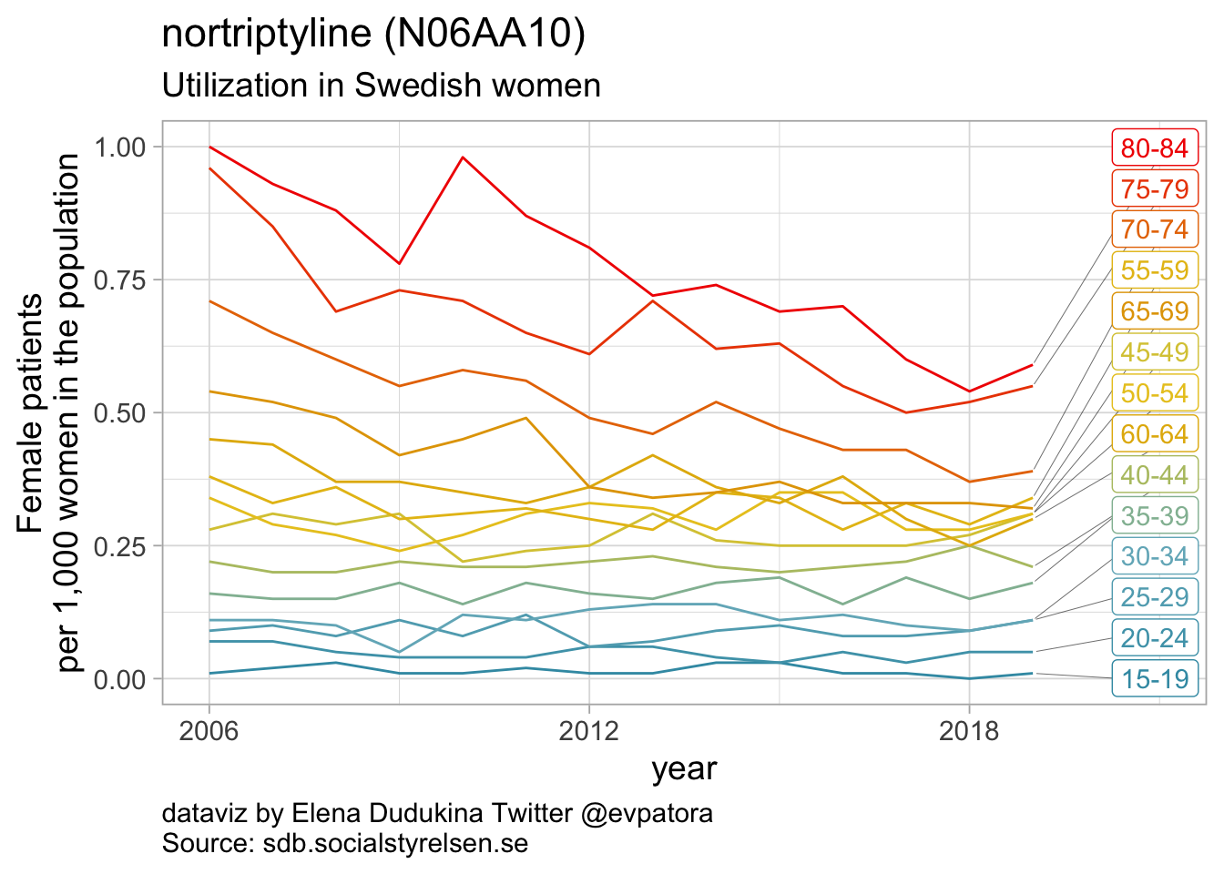
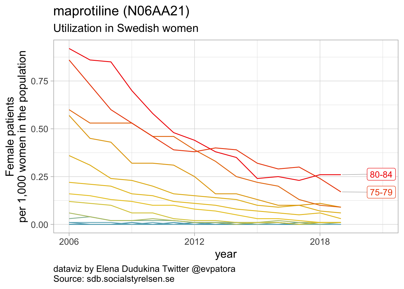
Non-selective monoamine reuptake inhibitors
- In 2019, utilization non-selective monoamine reuptake inhibitors (apart from amitriptyline) was low with the rate of 1 or fewer women per 1000
- In 2019, utilization of amitriptyline was 33 women per 1000 women for age group 80-84 years and 2-10 women per 1000 women for age groups between 15 and 34 years
list_plots_se[6:11]
## [[1]]
##
## [[2]]
##
## [[3]]
##
## [[4]]
##
## [[5]]
## Warning: ggrepel: 12 unlabeled data points (too many overlaps). Consider
## increasing max.overlaps
##
## [[6]]
data_se %>%
  filter(str_detect(ATC, "N06AB\\d{2}") & year== 2019) %>%
  group_by(ATC, ATC_label) %>%
  summarise(across(`Patienter/1000 invånare`, max)) %>%
  mutate(`Patienter/1000 invånare` = round(`Patienter/1000 invånare`, 0))
## # A tibble: 6 × 3
## # Groups:   ATC [6]
##   ATC     ATC_label    `Patienter/1000 invånare`
##   <chr>   <chr>                            <dbl>
## 1 N06AB03 fluoxetine                          24
## 2 N06AB04 citalopram                          59
## 3 N06AB05 paroxetine                           6
## 4 N06AB06 sertraline                          51
## 5 N06AB08 fluvoxamine                          0
## 6 N06AB10 escitalopram                        32
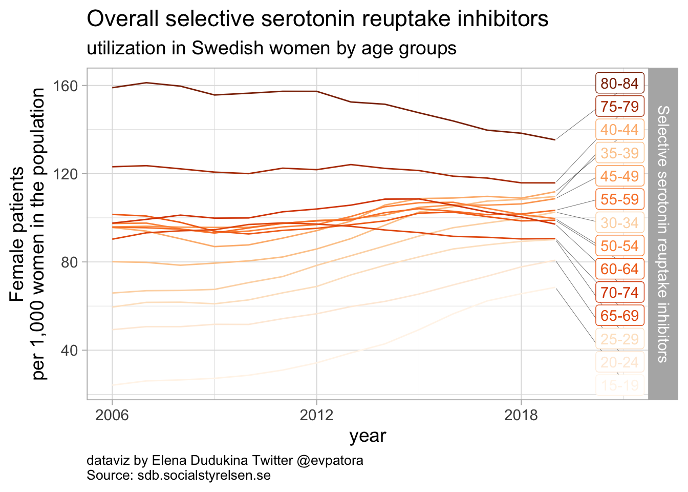
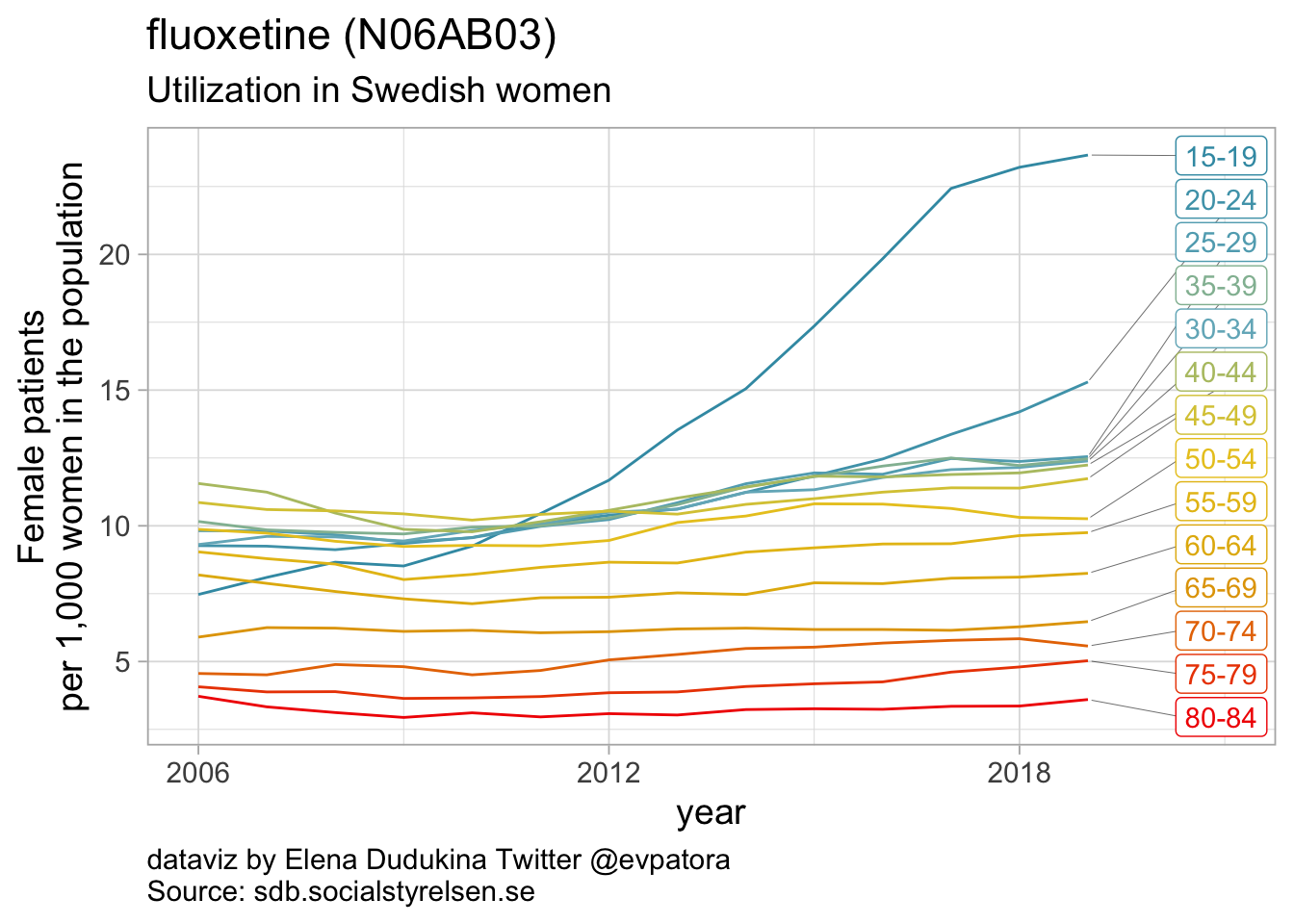
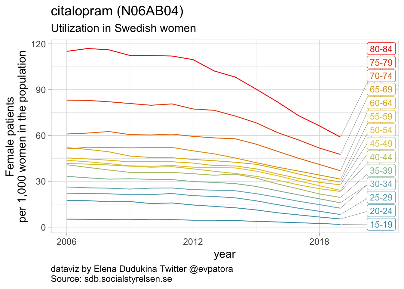
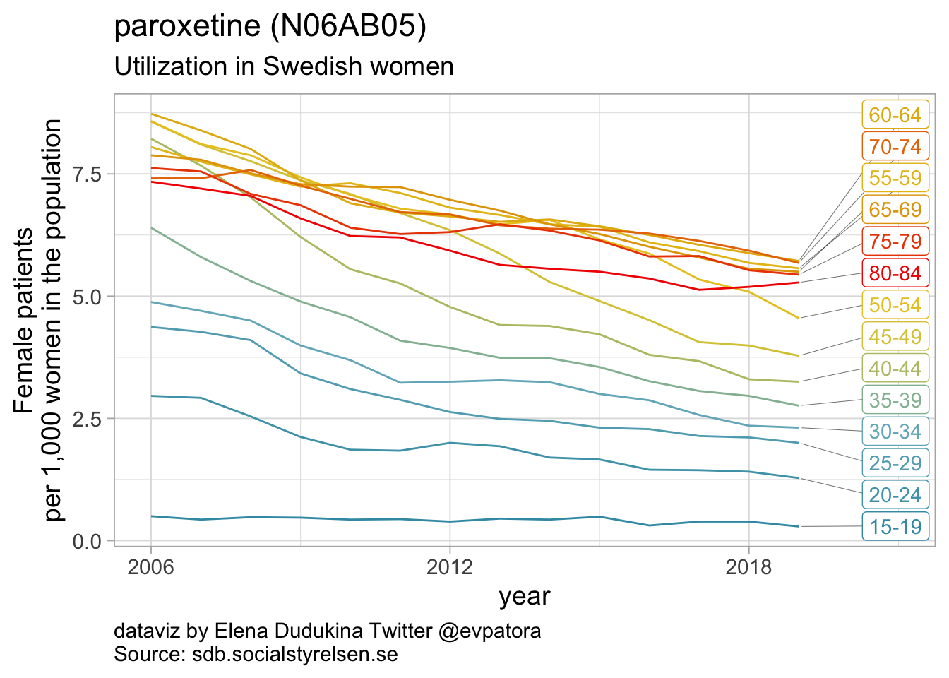
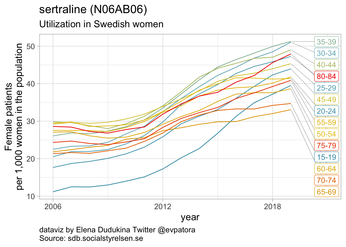
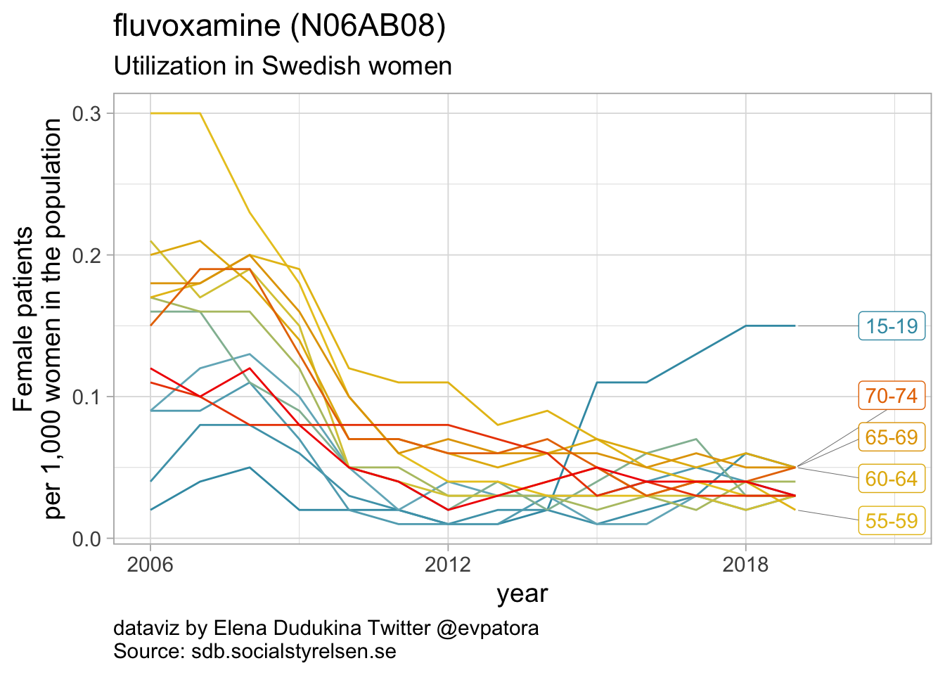
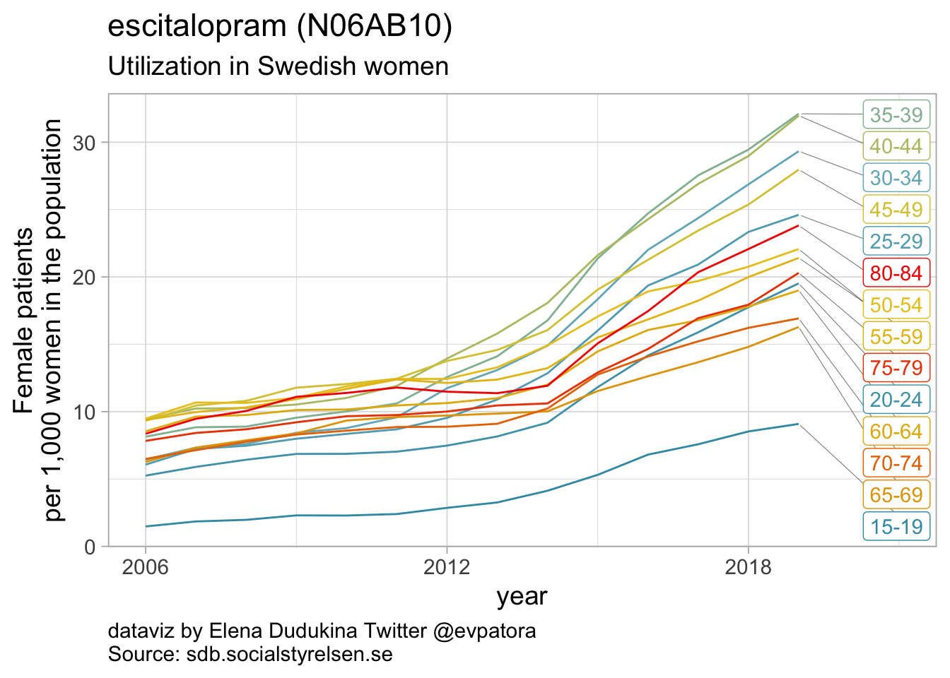
Selective serotonin reuptake inhibitors
- In 2019, the highest utilization rates were observed for citaprolam (59 per 1000 women) and for sertaline (51 per 1000 women)
- Utilization of fluoxetine was increasing over time among girls and young women aged between 15 and 19 years, and the highest utilization rate was observed in 2019 (24 per 1000 women)
- Utilization of escitalopram was increasing over time for all age groups; in 2019 the highest utilization was observed for women between 35 and 44 years (32 per 1000 women)
data_se %>%
  filter(str_detect(ATC, "N06AG\\d{2}") & year== 2019) %>%
  group_by(ATC, ATC_label) %>%
  summarise(across(`Patienter/1000 invånare`, max)) %>%
  mutate(`Patienter/1000 invånare` = round(`Patienter/1000 invånare`, 2))
## # A tibble: 1 × 3
## # Groups:   ATC [1]
##   ATC     ATC_label   `Patienter/1000 invånare`
##   <chr>   <chr>                           <dbl>
## 1 N06AG02 moclobemide                      0.24
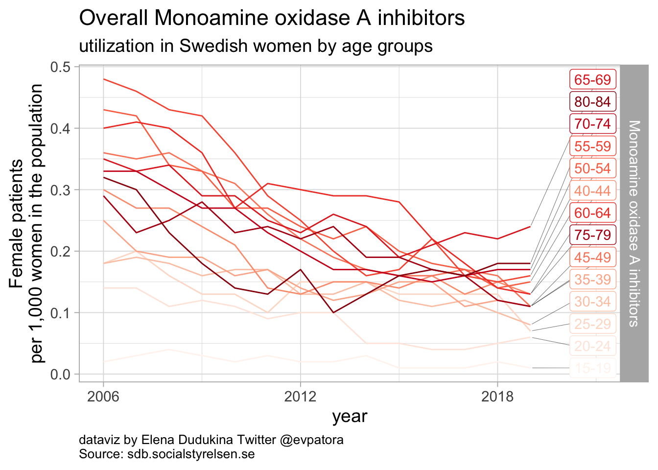
Monoamine oxidase A inhibitors
- The rate of moclobemide utilization was low (< 1 per 1000 women) for all age groups
data_se %>%
  filter(str_detect(ATC, "N06AF\\d{2}") & year == 2019) %>%
  group_by(ATC, ATC_label) %>%
  summarise(across(`Patienter/1000 invånare`, max)) %>%
  mutate(`Patienter/1000 invånare` = round(`Patienter/1000 invånare`, 2))
## # A tibble: 3 × 3
## # Groups:   ATC [3]
##   ATC     ATC_label       `Patienter/1000 invånare`
##   <chr>   <chr>                               <dbl>
## 1 N06AF01 isocarboxazid                        0
## 2 N06AF03 phenelzine                           0.03
## 3 N06AF04 tranylcypromine                      0.04
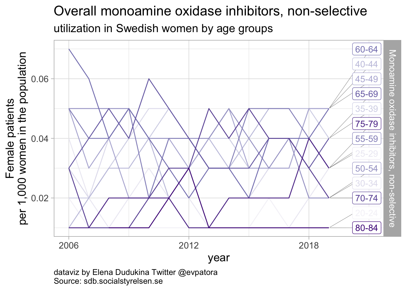
Non-selective monoamine oxidase inhibitors
- Utilization rate was very low for women of all investigated age groups
list_plots_se[13:21]
## [[1]]
##
## [[2]]
##
## [[3]]
##
## [[4]]
##
## [[5]]
##
## [[6]]
## Warning: ggrepel: 3 unlabeled data points (too many overlaps). Consider
## increasing max.overlaps
##
## [[7]]
##
## [[8]]
##
## [[9]]
data_se %>%
  filter(str_detect(ATC, "N06AX\\d{2}") & year == 2019) %>%
  group_by(ATC, ATC_label) %>%
  summarise(across(`Patienter/1000 invånare`, max)) %>%
  mutate(`Patienter/1000 invånare` = round(`Patienter/1000 invånare`, 0))
## # A tibble: 16 × 3
## # Groups: ATC [16]
## ATC ATC_label `Patienter/1000 invånare`
## <chr> <chr> <dbl>
## 1 N06AX01 oxitriptan 0
## 2 N06AX02 tryptophan 0
## 3 N06AX03 mianserin 3
## 4 N06AX05 trazodone 0
## 5 N06AX06 nefazodone 0
## 6 N06AX11 mirtazapine 112
## 7 N06AX12 bupropion 10
## 8 N06AX14 tianeptine 0
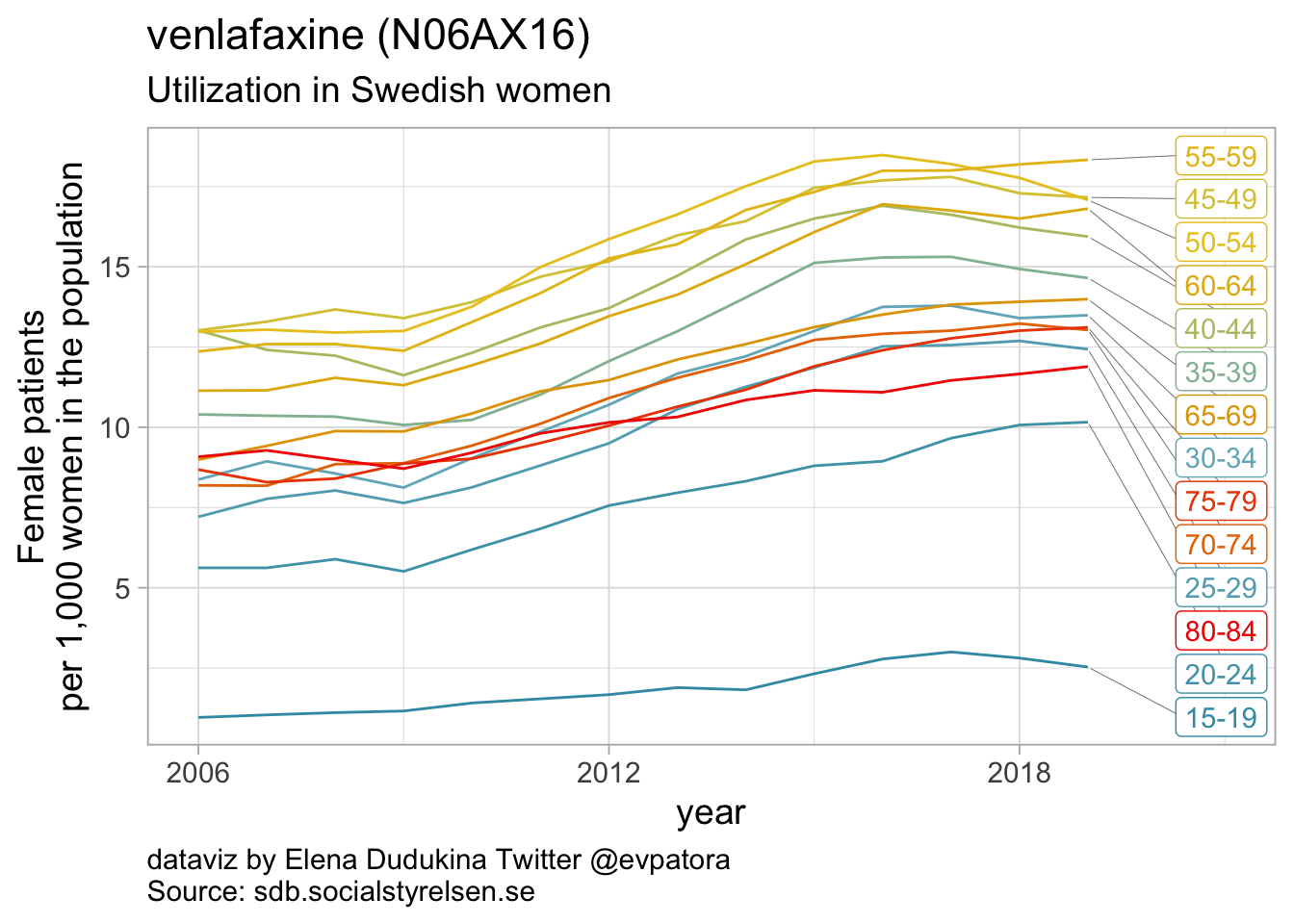
## 9 N06AX16 venlafaxine 18
## 10 N06AX17 milnacipran 0
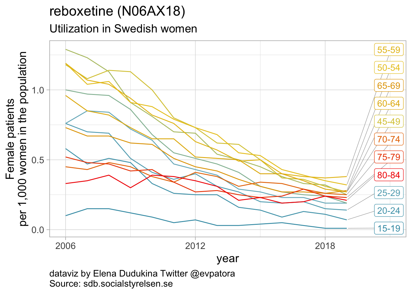
## 11 N06AX18 reboxetine 0
## 12 N06AX21 duloxetine 15
## 13 N06AX22 agomelatine 1
## 14 N06AX23 desvenlafaxine 0
## 15 N06AX24 vilazodone 0
## 16 N06AX26 vortioxetine 5
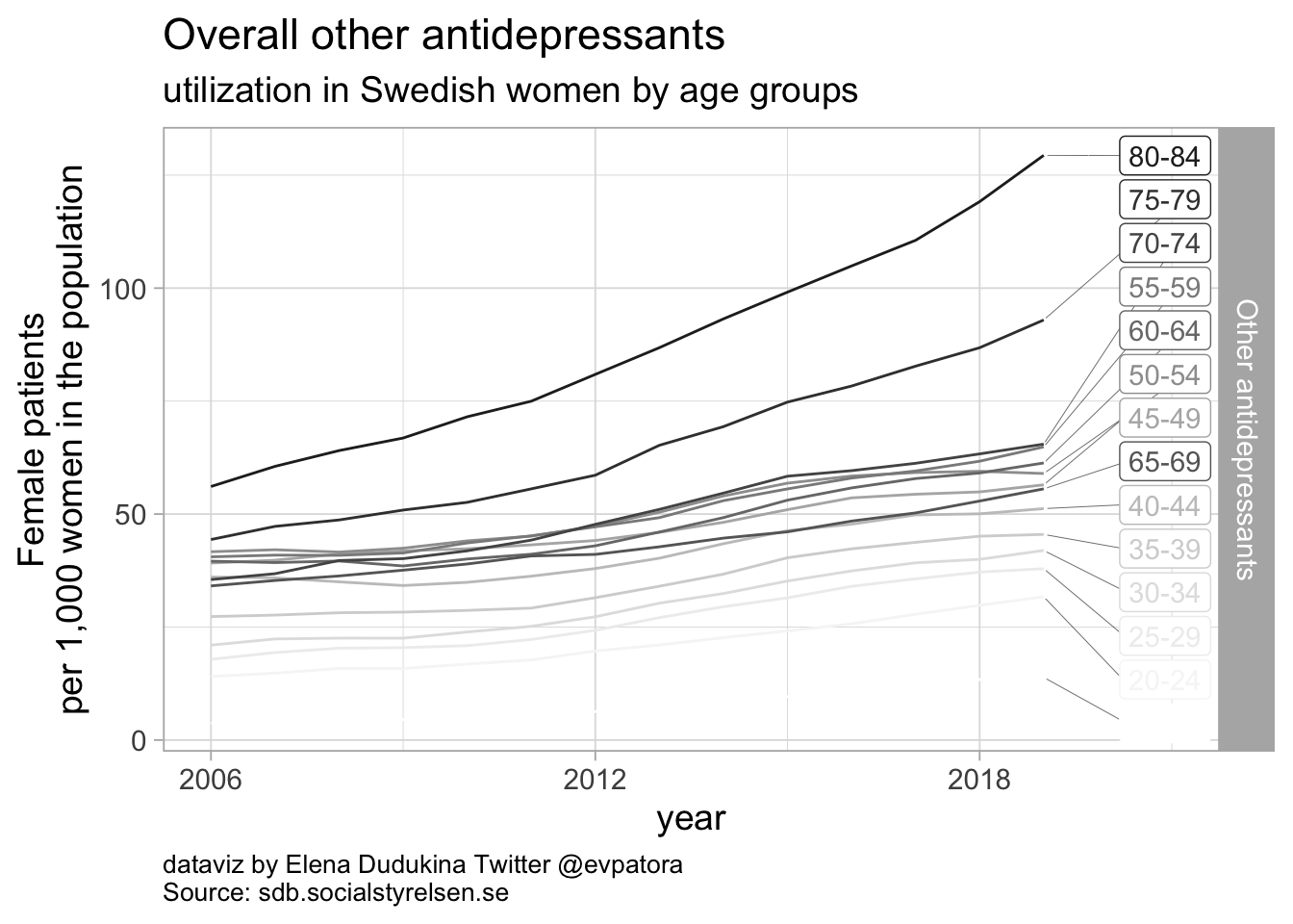
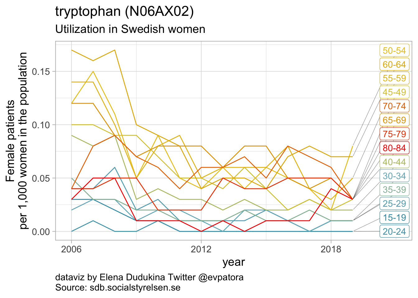
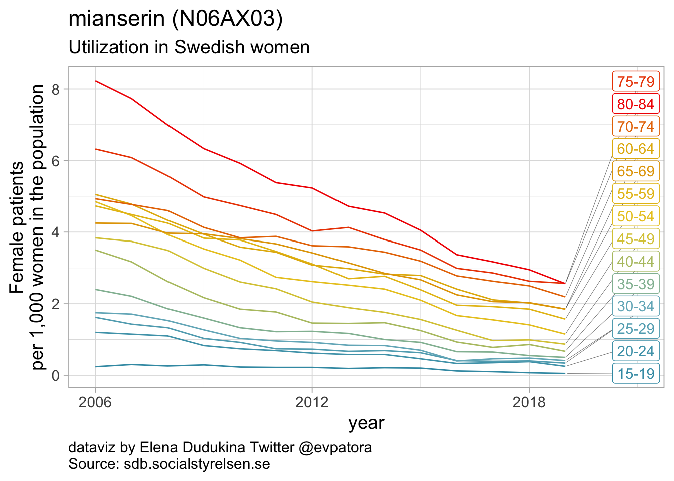
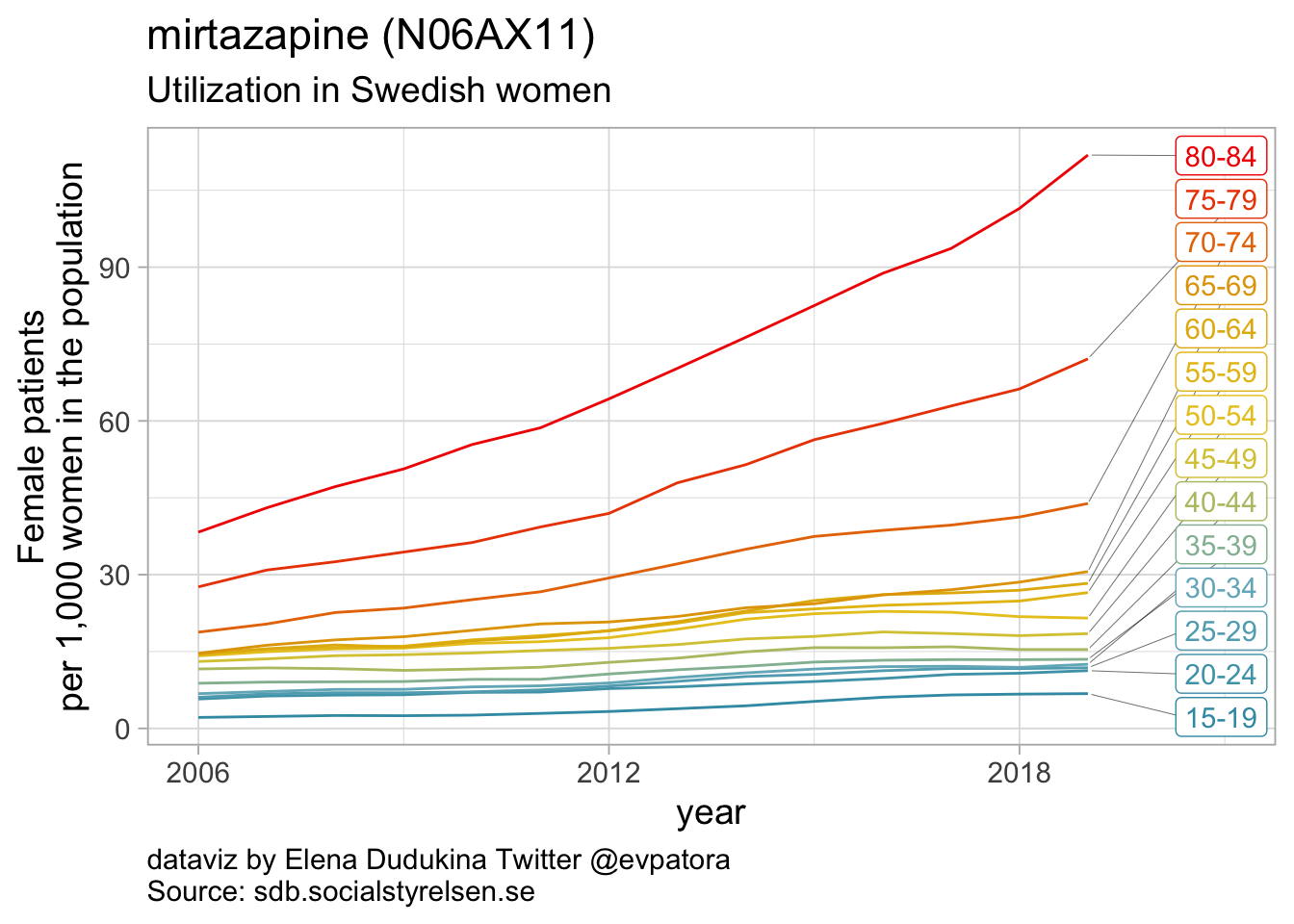
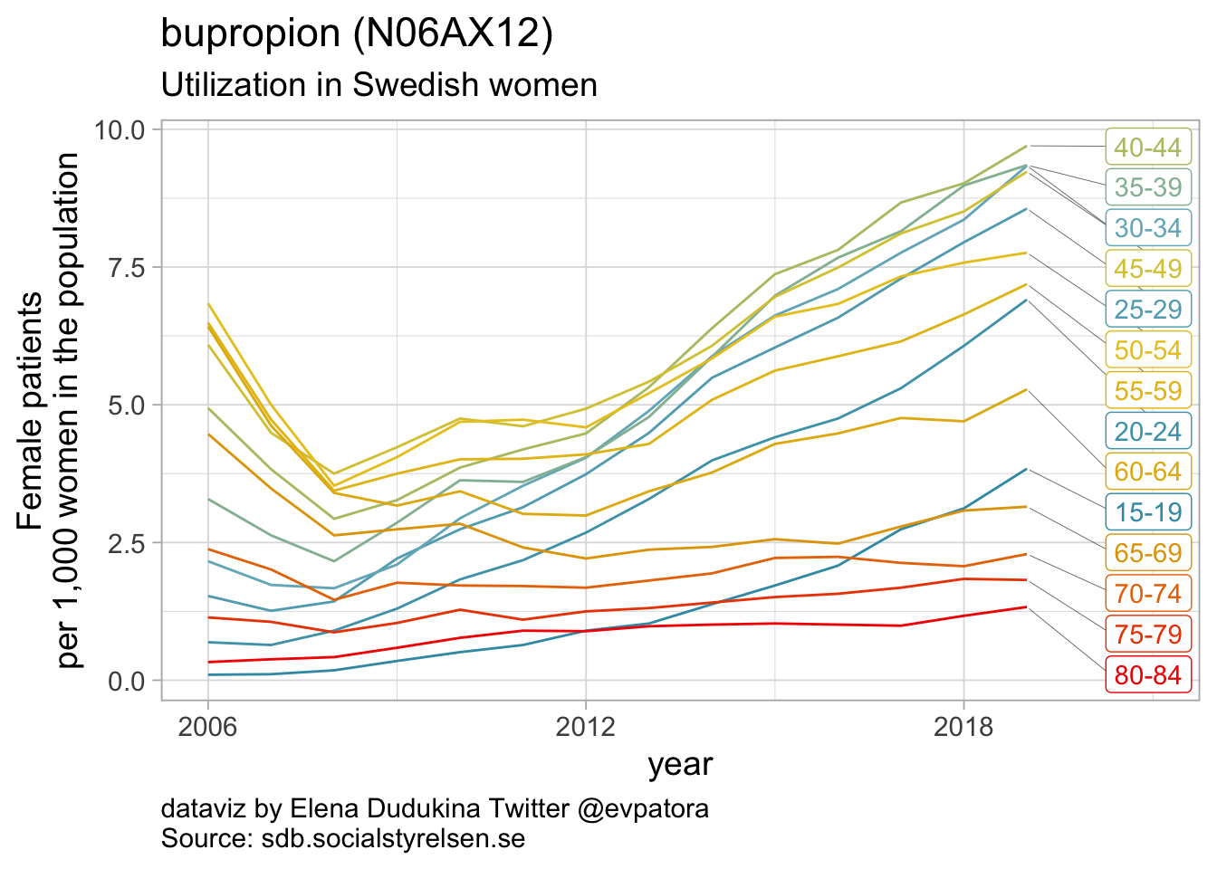
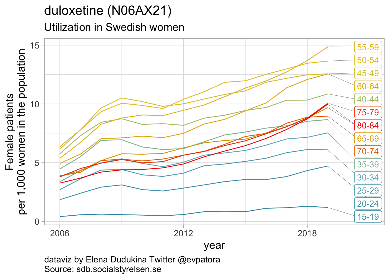
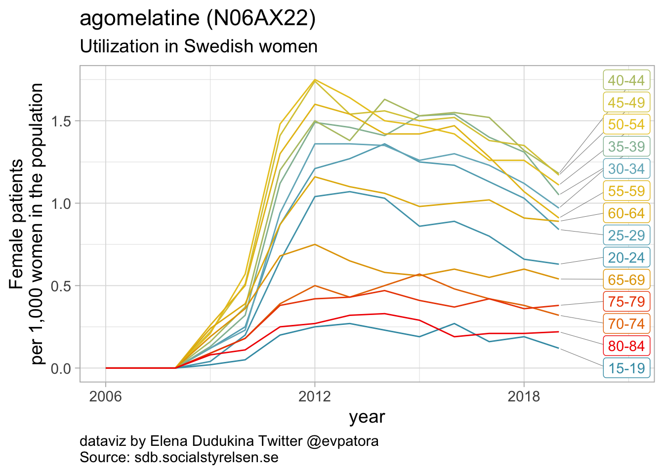
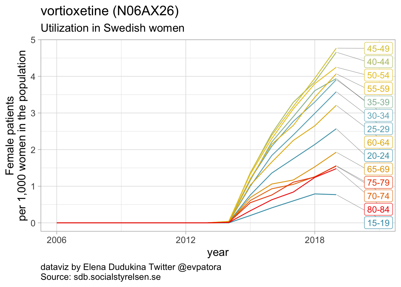
Other antidepressants utilization
- In 2019, mirtazapine utilization rate was 112 per 1000 women in the age group 80-84 years; utilization rate was increasing over time for the older age groups
- In 2019, bupropion utilization was ~10 per 1000 women in each of the age groups 35-39 years, 40-44 years, 45-49 years
- Utilization rate of duloxetine was increasing over time and in 2019 was the highest for women in the age group 55-59 years (15 women per 1000)
Major data caveats
- The data do not include medicines that are sold without prescription
- No data on indication
All feedback is very welcome and appreciated! 🤓