Drug utilization in Sweden and Denmark
Part I
Nordic open access databases
Nordic countries have databases with national aggregated data on, e.g. drug utilization, openly available. These databases are a great asset - you can investigate national trends for your curiosity or for research.
The databases are easily accessible and well-maintained. In this blog post, I will be taking a look at the Swedish aggregated drug utilization database.
Why I wrote this post?
The databases have a lot of useful features incorporated in a web interface, however it is not always sufficiently flexible to satisfy certain research tasks (in my personal experience). Ticking boxes is fun but - oh no - I selected one age category more than I intended, start again…🙈 It may be a frustrating experience when you need a quick and efficient check 👀 or when you perform multiple checks, for which reproducibility matters a lot.
What this post will cover?
This post (Part I) will be focused on Swedish national trends of antidepressants, antipsychotics, anxiolytics, and sedatives utilization in women. I compare Swedish and Danish national trends of utilization of these medications in part II.🇪
library(tidyverse)
library(magrittr)
library(wesanderson)
# I will keep only ATC codes I am interested in
regex_antidepress <- "^N06A$"
regex_antipsych <- "^N05A$"
regex_anxiolyt <- "^N05B$"
regex_sedat <- "^N05C$"

# combine all ATC codes in one regex string
all_regex <- paste(regex_sedat, regex_antipsych, regex_antidepress, regex_anxiolyt, sep = "|")
Data source
I use “CSV Statistics Database - Medicines 2006–2019” data from here.
Let’s go!
I will store .csv data files as a list and will name each element inside the list according to .csv file name.
# name the list elements according the name of downloaded .csv files
# path_se is your path with the downloaded and unzipped .csv files
file_names_se <- list.files(path = path_se, pattern = ".csv")

# load the data files
all_files_se <- map(file_names_se, ~read_delim(file = paste0(path_se, .x), trim_ws = T, delim = ";")) %>%
  # I expect that formatting of numbers in the files may not be standard; I re-format all columns to character type to deal with numbers' formatting later
  map(~mutate_all(.x, as.character))
The files containing the drug utilization per year include columns:
- Characteristic
- Year
- Region
- ATC
- Sex
- Age
- Value
all_files_se[[1]] %>% slice(1:5)
## # A tibble: 5 x 7
## Mått År Region `ATCkod` Kön Ålder Värde
## <chr> <chr> <chr> <chr> <chr> <chr> <chr>
## 1 3 2006 0 TOTALT 1 1 560858
## 2 3 2006 0 TOTALT 1 2 413587
## 3 3 2006 0 TOTALT 1 3 415480
## 4 3 2006 0 TOTALT 1 4 474248
## 5 3 2006 0 TOTALT 1 5 444933
# Note the region coded as integer 0, 1, 2
Before moving forward, I want to combine drug utilization data with these meta-data files.
# age
all_files_se[[71]] %>% slice(1:5)
## # A tibble: 5 x 2
##   Ålder Text
##   <chr> <chr>
## 1 1     0-4
## 2 2     5-9
## 3 3     10-14
## 4 4     15-19
## 5 5     20-24
# ATC codes
all_files_se[[72]] %>% slice(1:5)
## # A tibble: 5 x 2
##   ATC    Text
##   <chr>  <chr>
## 1 TOTALT Samtliga (A - V)
## 2 A      Matsmältningsorgan och ämnesomsättning
## 3 A01    Medel vid mun- och tandsjukdomar
## 4 A01A   Medel vid mun- och tandsjukdomar
## 5 A01AA  Medel mot karies
# Sex
all_files_se[[73]] %>% slice(1:5)
## # A tibble: 3 x 2
##   Kön   Text
##   <chr> <chr>
## 1 1     Män
## 2 2     Kvinnor
## 3 3     Båda könen
# Characteristic/stats
all_files_se[[74]] %>% slice(1:5)
## # A tibble: 5 x 2
##   Mått  Text
##   <chr> <chr>
## 1 1     Antal patienter
## 2 2     Patienter/1000 invånare
## 3 3     Antal expedieringar
## 4 4     Expedieringar/1000 invånare
## 5 9     Befolkning
# Region
all_files_se[[75]] %>% slice(1:5)
## # A tibble: 5 x 2
##   Region Text
##   <chr>  <chr>
## 1 00     Riket
## 2 01     Stockholms län
## 3 03     Uppsala län
## 4 04     Södermanlands län
## 5 05     Östergötlands län
# Note the region coded as 00, 01, 02 in the meta-data file and 0, 1, 2 in the files with stats
Combining data with meta-data
I am not speaking Swedish and it takes a moment to remember what some of the columns mean and which values are sensible; therefore, I do some re-coding.
# recode regions so that the coding in the meta-data file matches the stats data
all_files_se[[75]] %<>% mutate(Region = as.character(as.numeric(Region)))
# combine with meta-data
data_se <- bind_rows(all_files_se[c(1:70)]) %>%
  # join with age groups labels
  left_join(all_files_se[[71]]) %>%
  # rename joined column to age_group
  rename(age_group = Text) %>%
  # rename ATCkod to ATC
  rename(ATC = 4) %>%
  # keep only ATC codes of interest
  filter(str_detect(string = ATC, pattern = all_regex)) %>%
  # join with drugs labels
  left_join(all_files_se[[72]]) %>%
  # rename joined column
  rename(drug = Text) %>%
  # join with sex labels
  left_join(all_files_se[[73]]) %>%
  # rename joined column
  rename(gender = Text) %>%
  # keep records on drug utilization in women
  filter(gender == "Kvinnor") %>%
  # join with characteristics' labels
  left_join(all_files_se[[74]]) %>%
  # rename characteristics' labels column
  rename(stat = Text) %>%
  # join with regions' labels column
  left_join(all_files_se[[75]]) %>%
  # rename regions' labels column
  rename(region_text = Text) %>%
  # keep stats for the whole country
  filter(region_text == "Riket") %>%
  # rename some of the columns in the dataset while selecting columns in the desired order
  select(year = År,
         region = region_text,
         ATC,
         values = Värde,
         age_group,
         drug,
         gender,
         stat)
# checking the data
data_se %>% slice(1:5)
## # A tibble: 5 x 8
##   year  region ATC   values age_group drug         gender  stat
##   <chr> <chr>  <chr> <chr>  <chr>     <chr>        <chr>   <chr>
## 1 2006  Riket  N05A  3      0-4       Neuroleptika Kvinnor Antal expedieringar
## 2 2006  Riket  N05A  138    5-9       Neuroleptika Kvinnor Antal expedieringar
## 3 2006  Riket  N05A  922    10-14     Neuroleptika Kvinnor Antal expedieringar
## 4 2006  Riket  N05A  6276   15-19     Neuroleptika Kvinnor Antal expedieringar
## 5 2006  Riket  N05A  13139  20-24     Neuroleptika Kvinnor Antal expedieringar
Reshaping into wide format
# pivot data into wide format so that each stat has its column
data_se %<>% pivot_wider(names_from = stat, values_from = values) %>%
  # format numbers using with dot as a decimal separator
  mutate(
    `Expedieringar/1000 invånare` = str_replace_all(string = `Expedieringar/1000 invånare`, pattern = ",", replacement = "."),
    `Patienter/1000 invånare` = str_replace_all(string = `Patienter/1000 invånare`, pattern = ",", replacement = "."),
    `Expedieringar/1000 invånare` = as.numeric(`Expedieringar/1000 invånare`),
    `Patienter/1000 invånare` = as.numeric(`Patienter/1000 invånare`)
  ) %>%
  # all to numeric
  mutate_at(vars(`Antal expedieringar`, `Antal patienter`, Befolkning, year), as.numeric)

data_se %>% slice(1:5)
## # A tibble: 5 x 11
##    year region ATC   age_group drug    gender `Antal expedieri… `Antal patiente…
##   <dbl> <chr>  <chr> <chr>     <chr>   <chr>              <dbl>            <dbl>
## 1  2006 Riket  N05A  0-4       Neurol… Kvinn…                 3                2
## 2  2006 Riket  N05A  5-9       Neurol… Kvinn…               138               39
## 3  2006 Riket  N05A  10-14     Neurol… Kvinn…               922              222
## 4  2006 Riket  N05A  15-19     Neurol… Kvinn…              6276             1209
## 5  2006 Riket  N05A  20-24     Neurol… Kvinn…             13139             2102
## # … with 3 more variables: Befolkning <dbl>, Expedieringar/1000 invånare <dbl>,
## #   Patienter/1000 invånare <dbl>
Age categories
I will work with age categories between 20 and 54 years.
# age categories: check distinct, keep ages of interest
ages_to_keep <- data_se %>%
  distinct(age_group) %>%
  filter(row_number() %in% 5:11) %>%
  pull()

ages_to_keep
## [1] "20-24" "25-29" "30-34" "35-39" "40-44" "45-49" "50-54"
# age_cat_1
age_cat_1 <- data_se %>%
  distinct(age_group) %>%
  filter(row_number() %in% 5) %>%
  pull()

age_cat_1
## [1] "20-24"
# age_cat_2
age_cat_2 <- data_se %>%
  distinct(age_group) %>%
  filter(row_number() %in% 6:7) %>%
  pull()

age_cat_2
## [1] "25-29" "30-34"
# age_cat_3
age_cat_3 <- data_se %>%
  distinct(age_group) %>%
  filter(row_number() %in% 8:9) %>%
  pull()

age_cat_3
## [1] "35-39" "40-44"
# age_cat_4
age_cat_4 <- data_se %>%
  distinct(age_group) %>%
  filter(row_number() %in% 10:11) %>%
  pull()

age_cat_4
## [1] "45-49" "50-54"
Final dataset
# final data
data_se %<>%
  filter(age_group %in% ages_to_keep) %>%
  # group by year and ATC code to aggregate into age categories
  mutate(
    age_cat = case_when(
      age_group %in% age_cat_1 ~ "20-24",
      age_group %in% age_cat_2 ~ "25-34",
      age_group %in% age_cat_3 ~ "35-44",
      age_group %in% age_cat_4 ~ "45-54",
      T ~ NA_character_
    )
  ) %>%
  # keep only relevant ages
  filter(! is.na(age_cat)) %>%
  # to count number of women who received a prescription per ATC code, per age group, per year
  group_by(ATC, year, age_cat) %>%
  mutate(
    # number of patients in the numerator
    numerator = sum(`Antal patienter`),
    # population size in the denominator; denominator includes women of particular age category per year
    denominator = sum(Befolkning),
    patients_per_1000_inhabitants = numerator / denominator * 1000
  ) %>%
  ungroup() %>%
  # keep ATC codes of interest only
  filter(str_detect(string = ATC, pattern = all_regex))

data_se %>% slice(1:5)
## # A tibble: 5 x 15
##    year region ATC   age_group drug    gender `Antal expedieri… `Antal patiente…
##   <dbl> <chr>  <chr> <chr>     <chr>   <chr>              <dbl>            <dbl>
## 1  2006 Riket  N05A  20-24     Neurol… Kvinn…             13139             2102
## 2  2006 Riket  N05A  25-29     Neurol… Kvinn…             19561             2539
## 3  2006 Riket  N05A  30-34     Neurol… Kvinn…             27854             3330
## 4  2006 Riket  N05A  35-39     Neurol… Kvinn…             40778             4148
## 5  2006 Riket  N05A  40-44     Neurol… Kvinn…             57630             5328
## # … with 7 more variables: Befolkning <dbl>, Expedieringar/1000 invånare <dbl>,
## #   Patienter/1000 invånare <dbl>, age_cat <chr>, numerator <dbl>,
## #   denominator <dbl>, patients_per_1000_inhabitants <dbl>
A wrapper around the plotting function
Results
Antidepressants
list_plots_se[[1]]
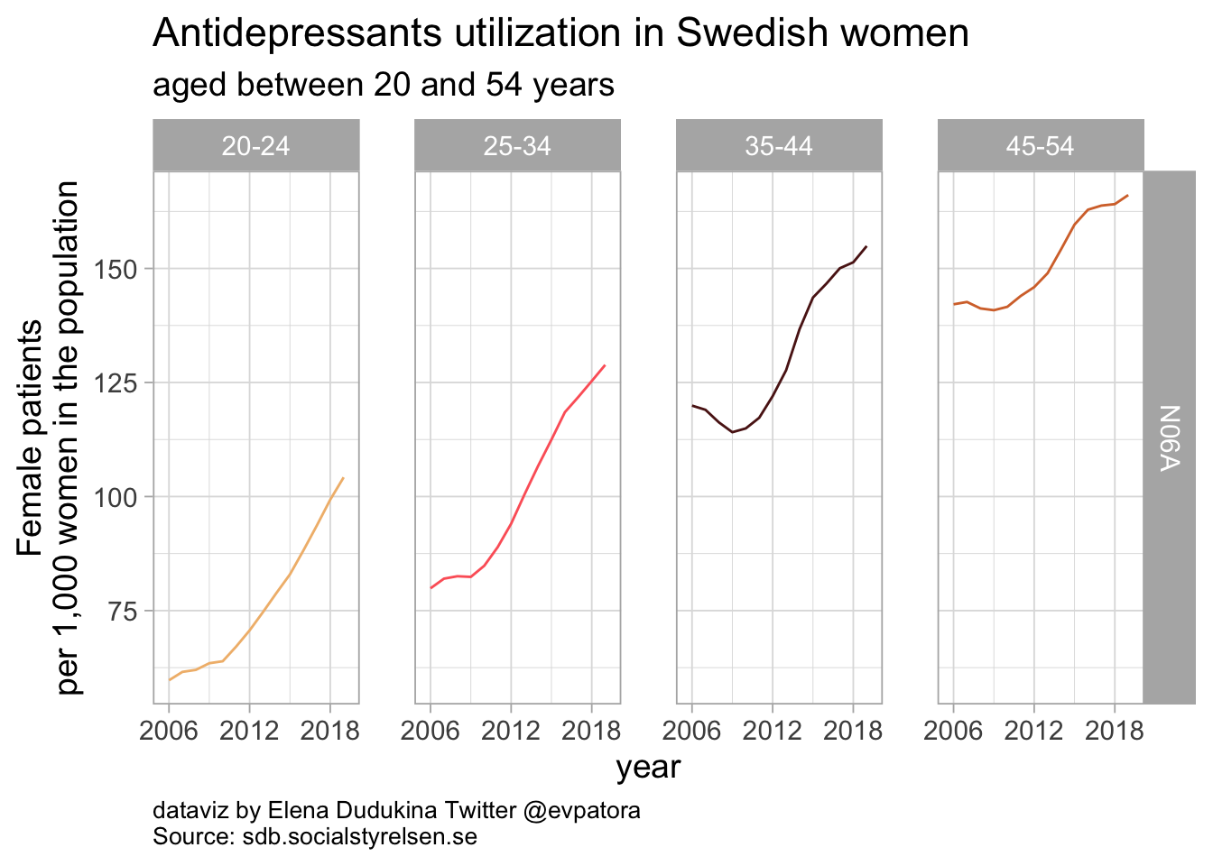
Antidepressants utilization in Swedish women was increasing starting in 2010. In 2019, 104 Swedish women per 1000 female inhabitants aged between 20-24 had a prescription of any antidepressant; 166 Swedish women aged between 45 and 54 years per 1000 female inhabitants in this age category received any antidepressant prescription.
Antipsychotics
list_plots_se[[2]]
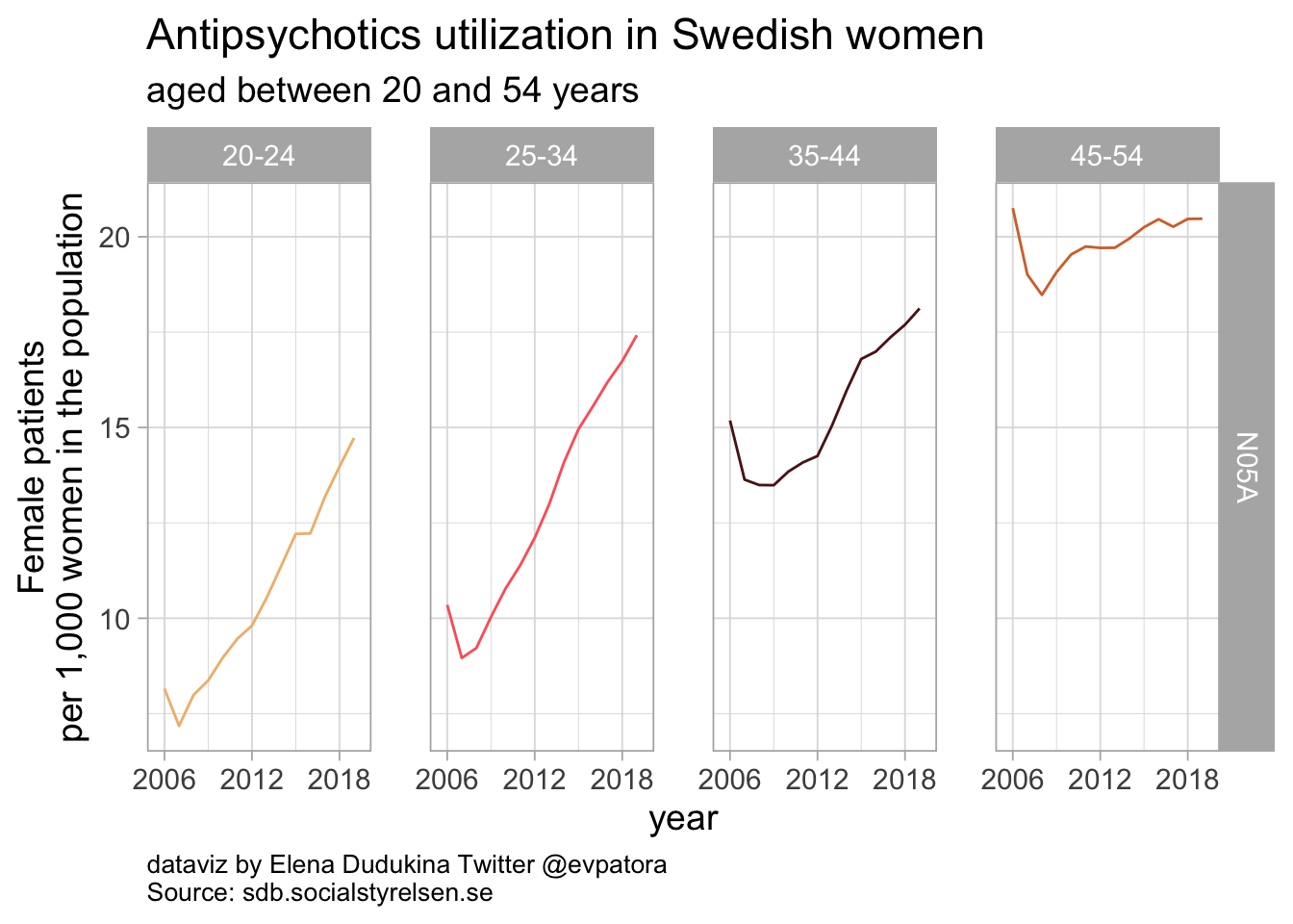
Antipsychotics utilization among Swedish women has risen sharply since 2007 for women in the age categories 20-24 years and 25-34 years. In 2019, 15 Swedish women per 1000 aged between 20-24 years, 17 Swedish women per 1000 aged between 25-34 years, 18 Swedish women per 1000 aged between 35-44 years, and 21 Swedish women per 1000 aged between 45-54 years received antipsychotics prescription.
Anxiolytics
list_plots_se[[3]]
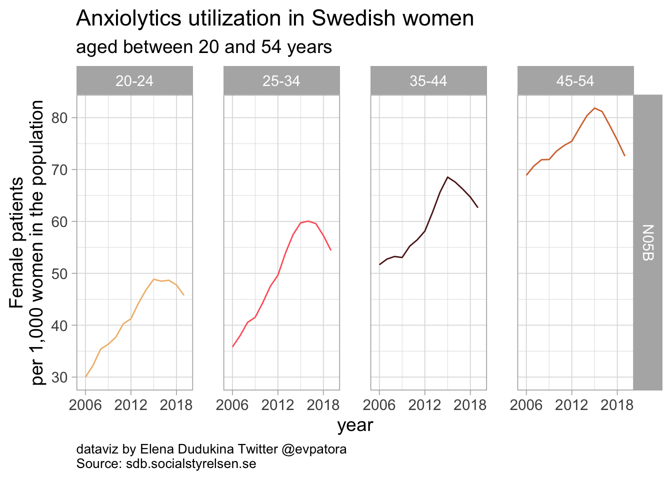
Anxiolytics utilization among Swedish women between 20 and 54 years of age was increasing from the beginning of medication utilization data recording in 2006. Starting in 2015, the rates of anxiolytics utilization was decreasing in women of all investigated age categories. In 2019, anxiolytics utilization varied between 46 women per 1000 in age category 20-24 years and 73 women per 1000 in age category 45-54 years.
Sedatives
list_plots_se[[4]]
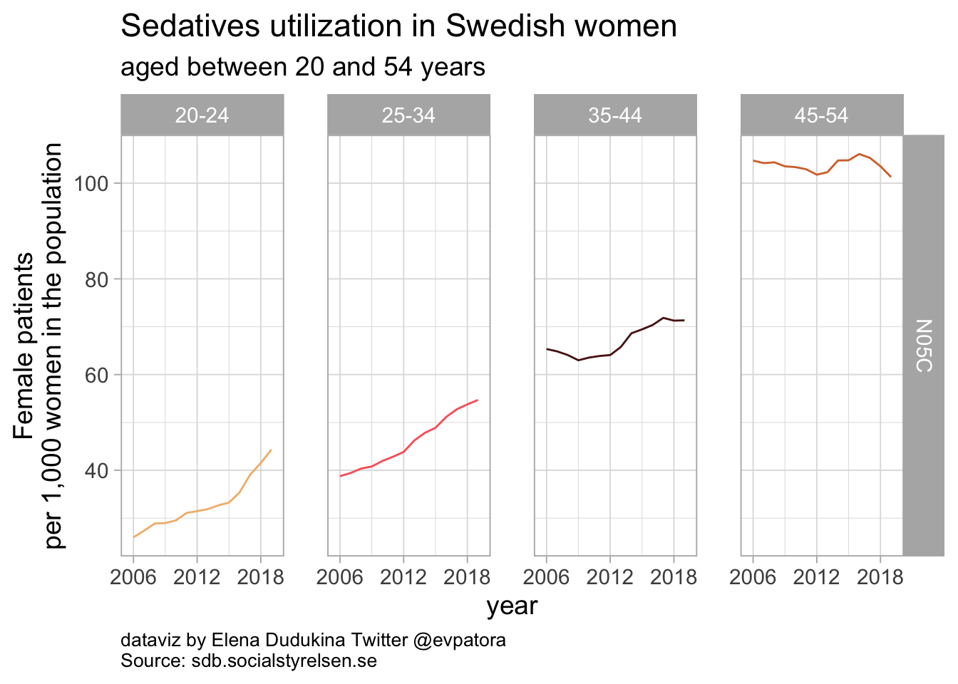
Sedatives utilization among Swedish women was between 44 women per 1000 in age category 20-24 years and 101 women per 1000 in age category 45-54 years. The rates of sedatives utilization remained nearly unchanged between 2006 and 2019 for women aged 45-54 years and was increasing among women between 20 and 44 years of age.
Data caveats
- The data do not include medicines that are sold without prescription
- No data on indication. Medication with the same ATC code with distinct indications will be aggregated
- “Number of patients” is the number of individuals who received a drug prescription at least once during the calendar year. For some medications, the “number of patients” can exceed the actual size of the given population
- The same individual may receive several prescriptions for different medications and therefore when summing over several drug groups, the same individual will be counted several times
The whole list of aggregated data caveats to keep in mind for Swedish drug utilization data can be found here.
Please leave your comments or questions via your preferred social media. All feedback is very much appreciated ✌